(More) Inference, and Hypothesis Testing

Agenda

Definitions, standard errors, confidence intervals for proportions
Hypothesis testing (is a particular value for the true parameter plausible?)
Differences in means and proportions

Estimating Proportions

Proportions are just means of binary (0/1) variables:

Sample:

Party	D	R
Dem	1	0
Rep	0	1
Dem	1	0
Dem	1	0
Rep	0	1

(3/5 are Dem)

Sample proportion: \[\widehat{p} = \frac{\text{total voting Dem}}{n} = \frac{1}{n}\sum_{i=1}^n D_i\] \[= \frac{1}{5}\times (1+0+1+1+0) = 3/5\]

This is just the sample mean of the 0/1 variable $D$ at left.

Standard error for a proportion

Standard error for a sample proportion is still \[ \sqrt{\frac{\text{estimated population variance}}{n}}, \] just like for a sample mean
But we have a simpler formula: \[s_{\widehat{p}} = \sqrt{\left(\frac{\widehat{p}(1-\widehat{p})}{n}\right)}\]

Political Polling: Confidence Interval

In a sample of 1,100 voters, 531 suport the Democratic candidate. What proportion of all voters support the Democratic candidate?

Sample proportion: $\widehat{p} = \frac{531}{1100} = 0.483$ (48.3%)
Standard error: $s_{\widehat{p}} = \sqrt{\frac{\widehat{p}(1-\widehat{p})}{n}} = \sqrt{\frac{0.483 \times 0.517}{1100}} = 0.015$
95% confidence interval: $0.483 \pm 2(0.015) = [0.453, 0.513]$

48.3% ± 3% = [45.3%, 51.3%] of voters support the Democratic candidate

Hypothesis Testing

Hypothesis tests

Confidence intervals give us the range of plausible values that are consistent with the data in hand
Often specific values are more interesting than others (like average ROE in our SAP example)
Hypothesis testing asks: How plausible or implausible is one specific value of the true parameter

Triangle Test

Mexican Coke vs American Coke

Mexican Coke uses cane sugar
American Coke uses high fructose corn syrup
Mexican Coke has devoted fans willing to pay premium prices
But can people actually taste the difference?

Question:

Can consumers detect a difference? (Common question when changing ingredients/suppliers/processes!)

Should Coca-Cola switch to cane sugar despite higher costs?

How the Triangle Test Works

The Setup:

Present 3 samples to each participant
2 samples are identical, 1 is different
Ask: “Which one is the odd one out?”
Even with no detectable difference, participants must choose
By pure guessing, each person has 1/3 chance of being correct
If people can detect differences, correct rate should exceed 1/3

Triangle Test: What Do We Expect?

Suppose we test 36 participants and there’s truly no difference. How many would we expect to get the right answer?

About 12 (one-third of 36). If there’s no difference, would 11 be surprising? How about 15? Or 24?

The question: Where do we draw the line between “could be chance” and “strong evidence of real difference”?

Instructions

In groups of 3:

Get 6 cups (two sets of 3 with distinct colors)
Choose one person to administer the test; the other two are panelists
For each panelist:
1. Pour the “odd sample out” (cane sugar) into a randomly selected cup
2. Write down the correct colors
3. Fill the other two cups with the regular samples
Repeat for the other panelist while the first is making their selection

Hypothesis Testing: The Four Steps

Specify a null hypothesis
- “These two products are perceptibly identical”
- $H_0: p = 1/3$ (everyone is guessing)
Compute a test statistic
- Measures strength of evidence against the null
- t-statistic: $t = \frac{\widehat{p} - 1/3}{s_{\widehat{p}}}$
Find distribution assuming null is true
- If $H_0$ is true, then $t \sim N(0,1)$
Quantify strength of evidence
- Compute p-value: probability of seeing results this extreme if null is true

Why “Null” Hypothesis?

The null hypothesis represents no effect, no difference, no relationship

Examples:

Triangle test: No perceptible difference ($p = 1/3$)
SAP profitability: No difference from industry average
New routing algorithm: No improvement in delivery times
Comparing two suppliers: No difference in defect rates

We always start here, even if we believe there is an effect/difference/relationship…

The Courtroom Analogy

Hypothesis testing is like putting the null hypothesis on trial:

Prosecutor: Convinced defendant is guilty (null is false)
Defendant’s mom: Convinced defendant is innocent (null is true)
Jury: Must presume innocence until proven guilty

Your role: Be an impartial juror

Start by presuming the null hypothesis is true (innocent)
Weigh the evidence against it
Only “convict” (reject null hypothesis) with sufficient evidence

Evidence: The t-statistic

\[t = \frac{\text{estimate} - \text{hypothesized value}}{\text{standard error}}\]

Measures deviation from hypothesized value in units of standard errors

Distribution of the t-stat

If the null is true, then each participant’s decision is an independent random variable:

\[ X_i = \begin{cases} 1 & \text{with probability } p = 1/3 \\ 0 & \text{with probability } (1-p) = 2/3 \end{cases} \] From the Central Limit Theorem, \[ \hat{p}\sim N(1/3, s^2_{\hat p}) \Rightarrow \frac{\hat p - 1/3}{s_{\hat p}} \sim N(0,1) \] (approximately)

Distribution of the t-stat

If null hypothesis is true: $t \sim N(0,1)$ (it’s a z-score)
If null hypothesis is false: $t$ has different expected value
Larger |t| = stronger evidence against null hypothesis (unlikely to get results like this by chance when it’s true)

Triangle Test Example: t-statistic

Scenario: 18 correct out of 36 participants

Sample proportion: $\widehat{p} = 18/36 = 0.5$
Standard error: $s_{\widehat{p}} = \sqrt{\frac{0.5 \times 0.5}{36}} = 1/12$
t-statistic: $t = \frac{0.5 - 1/3}{1/12} = \frac{1/6}{1/12} = 2.0$

Interpretation: Our estimate is 2 standard errors away from the null hypothesis value

The p-value

Definition: Probability of observing a test statistic at least as extreme as what we got, assuming the null hypothesis is true

For our triangle test with $t = 2.0$, under the null hypothsesis:

p-value = P(Z ≥ 2.0) when Z ~ N(0,1)
p-value ≈ 0.025 (2.5%)

Interpretation: If there’s truly no difference, only 2.5% of similar experiments would show 18+ correct answers

p-value Visualization

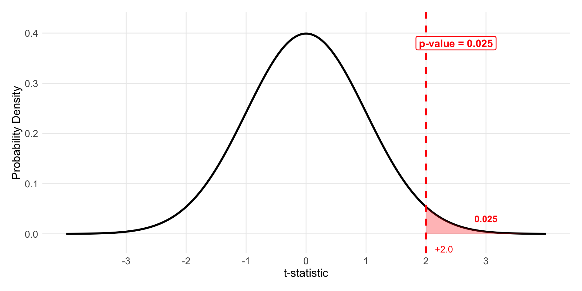
Figure 1: Computing the 1-tailed p-value for the triangle test with t-stat of 2.0

SAP Profitability: Hypothesis Test

Question: Are SAP customers as profitable as industry average?

Data: - Sample: 81 SAP customer firms - Sample mean ROE: 12.6% - Sample standard deviation: 25.7% - Industry average ROE: 15.7%

Null Hypothesis: - $H_0: \mu = 15.7\%$ (SAP customers have industry average profitability)

SAP Profitability: Test Calculation

Step 1: Standard error of sample mean \[s_{\bar{X}} = \frac{s}{\sqrt{n}} = \frac{25.7}{\sqrt{81}} = 2.86\%\]

Step 2: t-statistic \[t = \frac{\bar{X} - \mu_0}{s_{\bar{X}}} = \frac{12.6 - 15.7}{2.86} = \frac{-3.1}{2.86} = -1.08\]

Step 3: p-value For two-tailed test: p-value = P(|Z| ≥ 1.08) ≈ 0.28

SAP Profitability: p-value

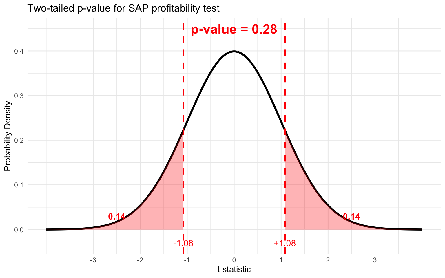
One vs Two-Tailed P-values

For the triangle test we only used the upper tail probability
If $p\neq 1/3$, then it must be bigger
For SAP, we used both tails
If $\mu\neq 15.7\%$, it could be bigger or smaller
If in doubt, use two tails like SAP – this is usually the better choice.

What the p-value is NOT

Common Misinterpretation: “p-value = 0.28 means there’s a 28% chance the null hypothesis is true”

This is WRONG!

p-value asks: “If the defendant were truly innocent, what’s the probability we’d see evidence this strong or stronger?” ($\Pr(\text{evidence}\mid \text{innocent})$)
NOT: “What’s the probability the defendant is innocent given this evidence?” ($\Pr(\text{innocent}\mid \text{evidence})$)

What the p-value is NOT

For SAP Example:

p-value = 0.28 means: “If SAP customers truly have industry-average profitability, there’s a 28% chance we’d see a random sample of 81 firms with a sample mean at least 3.1 percentage points away from 15.7%”
NOT: “There’s a 28% chance SAP customers have industry-average profitability”

Remember: The p-value assumes the null hypothesis is true to calculate the probability. It can’t tell us the probability that assumption is correct!

Hypothesis Testing as a Decision Problem

Common rule: Reject null hypothesis if p-value < $\alpha$ for some $\alpha$, usually 0.05.

p < 0.05: “Statistically significant” - reject null
p ≥ 0.05: “Not statistically significant” - fail to reject null

Hypothesis Testing as a Decision Problem

Important: “Fail to reject the null” ≠ “Accept null”

Like in court: Not guilty ≠ Innocent
We could fail to reject because the data are highly consistent with the null hypothesis or because variablity is large (e.g. due to small sample size)

Connection to Confidence Intervals

A 95% confidence interval contains exactly the values that would not be rejected in a hypothesis test at α = 0.05

SAP Example:

Sample mean: 12.6%
95% CI: [6.8%, 18.4%]
Industry average: 15.7%

Two hypothesis:

15.7% (in the 95% CI → Don’t reject)
20% (outside the 95% CI → Reject)

Why: All values in CI are within 2 standard errors of the estimate, so |t| < 2

CI and Hypothesis Test Connection

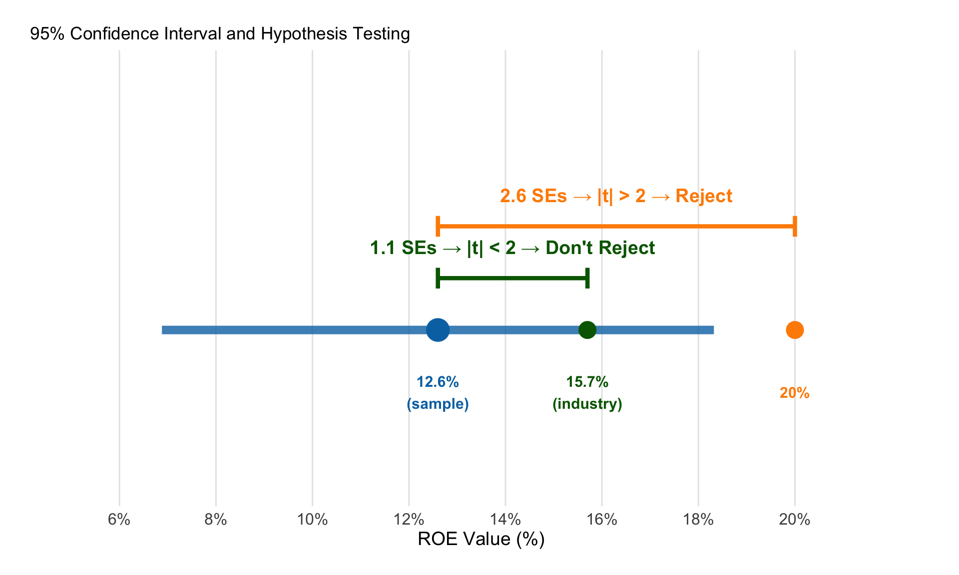
Comparing Groups

Comparing Two Groups

Many business questions involve comparing groups:

Which training program is more effective?
Do two suppliers have different defect rates?
Which website design converts better?
Are our customers more profitable than industry average?

We need methods to compare means and proportions between independent groups

Coding Bootcamp

Business Question: A tech company wants to choose between two coding training programs for new hires. Which is more effective?

Study Design: Employees randomly assigned to programs, then tested on standardized coding exercise

Data:

Intensive program: n=70, mean=129, SD=20
Standard program: n=50, mean=120, SD=25

Goal: Estimate difference in population means and test if we have strong evidence it isn’t zero

Differences in Means: Standard Error

When comparing two independent groups A and B:

Difference in sample means: $\bar{X}_A - \bar{X}_B$

Standard error of the difference: \[s_{\bar{X}_A - \bar{X}_B} = \sqrt{\frac{s_A^2}{n_A} + \frac{s_B^2}{n_B}}\]

where $s_A, s_B$ are sample standard deviations and $n_A, n_B$ are sample sizes

Coding Bootcamp: Analysis

Null hypothesis: $H_0: \mu_{A} - \mu_{B} = 0$ (no difference) v Step 1: Difference in means = 129 - 120 = 9 points

Step 2: Standard error of difference: \[s_{\bar{X}_A - \bar{X}_B} = \sqrt{\frac{20^2}{70} + \frac{25^2}{50}} = \sqrt{5.71 + 12.5} = 4.3\]

Coding Bootcamp: Analysis

Step 3: t-statistic: \[t = \frac{9 - 0}{4.3} = 2.09\]

Step 4: p-value ≈ 0.037 (two-tailed)

Coding Bootcamp: p-value

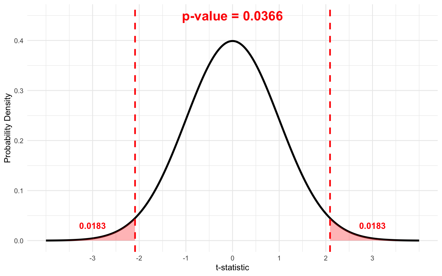
Differences in Means: Confidence Interval

Difference in sample means: $129 - 120 = 9$ points

95% confidence interval for difference: \[9 \pm 2(4.3) = [0.4, 17.6]\]

Interpretation: - All plausible values are positive (0.4 to 17.6 points) - Strong evidence intensive program is more effective on average

Differences in Means: The Decision

What should the company do? It depends!

What does an increase of 9 points (or as little as 0.4, or as many as 17.6) mean for job performance?
What do the programs cost?
What is the opportunity cost of the intensive?

Here are all the slides for the supplier quality example together:

Example: Supplier Quality Evaluation

Business Decision: Manufacturing company choosing between two suppliers for critical components

Data from 6-month evaluation:

Supplier A (Current): 15,000 parts tested, 180 defective (1.2% defect rate)
Supplier B (Premium): 15,000 parts tested, 120 defective (0.8% defect rate)

Differences in Proportions: Standard Error

When comparing two independent groups A and B:

Difference in sample proportions: $\hat{p}_A - \hat{p}_B$

Standard error of the difference: \[s_{\hat{p}_A - \hat{p}_B} = \sqrt{\frac{\hat{p}_A(1-\hat{p}_A)}{n_A} + \frac{\hat{p}_B(1-\hat{p}_B)}{n_B}}\]

where $\hat{p}_A, \hat{p}_B$ are sample proportions and $n_A, n_B$ are sample sizes

Estimate + Standard Error

Difference: $\hat{p}_A - \hat{p}_B = 0.012 - 0.008 = 0.004$ (0.4 percentage points)
Standard error: $s_{\hat{p}_A - \hat{p}_B} = \sqrt{\frac{0.012 \times 0.988}{15000} + \frac{0.008 \times 0.992}{15000}} = 0.00112$

Supplier Quality: Confidence Interval

95% confidence interval for difference in defect rates:

\[(\hat{p}_A - \hat{p}_B) \pm 2 \times s_{\hat{p}_A - \hat{p}_B}\]

\[0.004 \pm 2(0.00112) = 0.004 \pm 0.00224\]

\[[0.0018, 0.0062] \text{ or } [0.18\%, 0.62\%]\]

All plausible values are positive → strong evidence that Supplier A produces more defects

Estimate + Standard Error

Null hypothesis $H_0: p_A - p_B = 0$ (no difference in defect rates)

Difference: $\hat{p}_A - \hat{p}_B = 0.012 - 0.008 = 0.004$
Standard error: $s_{\hat{p}_A - \hat{p}_B} = 0.00112$
t-statistic: $t = \frac{0.004 - 0}{0.00112} = 3.57$
p-value $\approx$ 0.0004

The Decision Problem

OK, there’s a difference. What should the company do? They puurchase 50,000 parts a year, and:

Cost difference: Supplier B costs $150,000 more annually
Quality difference: Best guess, Supplier A produces ~200 more defective parts per year (0.4% of 50,000)
Defect cost: $450 per defective part

The Decision Problem

What do they save going with Supplier A (more defects)?

Best estimate (0.4% difference in defect rates):

Additional defects: 200 × $450 = $90,000
Net savings: $150,000 - 90,000 = 60,000

Worst case scenario (0.62% upper limit of CI):

Additional defects: 310 × $450 = $139,500
Net savings: $150,000 - 139,500 = 10,500

The Decision Problem

Even at the worst plausible quality difference from our confidence interval, Supplier A still saves money overall.
Statistical significance ≠ economic importance. Always ask whether a detected difference is large enough to change your business decision.

Key Takeaways

Confidence intervals show plausible values for parameters
Hypothesis testing asks if specific values are plausible
p-values measure strength of evidence against null hypothesis
Connection: 95% CI contains all values not rejected at α = 0.05
Practical significance ≠ statistical significance

Remember: Large samples can detect tiny differences that don’t matter practically!