Intro and Linear Regression Refresher

Introduction to the course

Answer two questions for me:

What is one thing you’re excited about for this class?

What is one thing you’re nervous or concerned about for this class?

Pass around your answers. Another student will read your responses, so everyone stays anonymous.

Canvas

Access at https://canvas.utexas.edu
Check out the home page for the weekly schedule and to meet the course staff
Make sure you can log in and are enrolled in STA 235 in Canvas

Class structure

Class will be synchronous and in person; class time will be divided between assessment, lecture, and practice
Understanding the concepts really only comes from practice; the course is designed to provide you with many opportunities!
Frequent assessments let you check your understanding

Grading

1000 total points allocated according to:

Component	Points
Pre-class prep (Perusall)	44
Class Participation (Instapoll)	86
Homework	195 (15 each)
Checkpoint Quizzes (13, 2 drops)	275 (25 each)
Mastery exams (2)	300 (200 each)
Data Storytelling	120 (20 + 120)

Pre-class prep

This is a fast-paced course, so it’s essential that you think about the material before class
We will use Perusall for pre-class reading assignments
Use Perusall to ask and answer your classmates questions, and share your knowledge, thoughts, and opinions
This will help you better understand the material and will help me gear class time to what topics you are having the most trouble with
Use the readings as a reference for study/homework too!

Pre-class prep

Pre-class readings are due 11:59PM the day before class
Grading is based on engagement
Each assignment is scored 0-4, but I will count a 3 or above (75%) as full credit (so don’t worry about your grade)

Class Participation

We will do regular check-ins and polls via Instapoll (clicker software on Canvas) on your mobile device or laptop
Answer 75% of questions (correctly or incorrectly) for full participation credit

Homework

Why homework? PRACTICE!
Homework helps you solidify your understanding of the material and prepare for checkpoint quizzes and mastery exams
Due at the end of your class day (11:59PM)
OK to work together, but try the problems on your own first.
Genereative AI is allowed, but don’t cheat yourself of valuable practice
Homework is autograded and you have three attempts. Start early so you can get help!

Checkpoint Quizzes

Research shows frequent, low-stakes assessment is better for learning than high-stakes exams alone
Checkpoint quizzes provide regular feedback on how you’re doing
You may bring one index card of notes (3.5 by 5 inch) and use statistical software (RStudio on Posit Cloud)
There are no makeup quizzes (except for documented emergencies).

Mastery Exams

Two Mastery Exams covering the first and second half of the course
One 8.5 x 11” sheet of notes for reference, and you can use RStudio on Posit Cloud to do calculations.
Mastery Exam A will be held 7-9 PM on either March 9 or 10 (your choice)
Mastery Exam B will be held during finals

Statistical computing

We will use R for statistical analysis throughout the course
This is industrial-strength, state-of-the-art, and free software for statistical computing
We will access R through the RStudio graphical interface
- Exams and quizzes: RStudio on Posit Cloud
- Homework and practice: RStudio on Posit Cloud or your laptop

Getting help

My office hours
TA/CA office hours (schedule on Canvas this week)
Post questions in readings in Perusall (for questions about the readings)
Post questions in group chats in Perusall (for general questions about the course, or homework questions)
Message me via Canvas

Linear Regression Refresher

Data description:

Subset of single family home sales in 3 Austin zipcodes
Variables include location, size, number of bedrooms, number of bathrooms (more)
Focus on predicting sale price from number of bedrooms, and living area/size as a first example

Price vs bedrooms

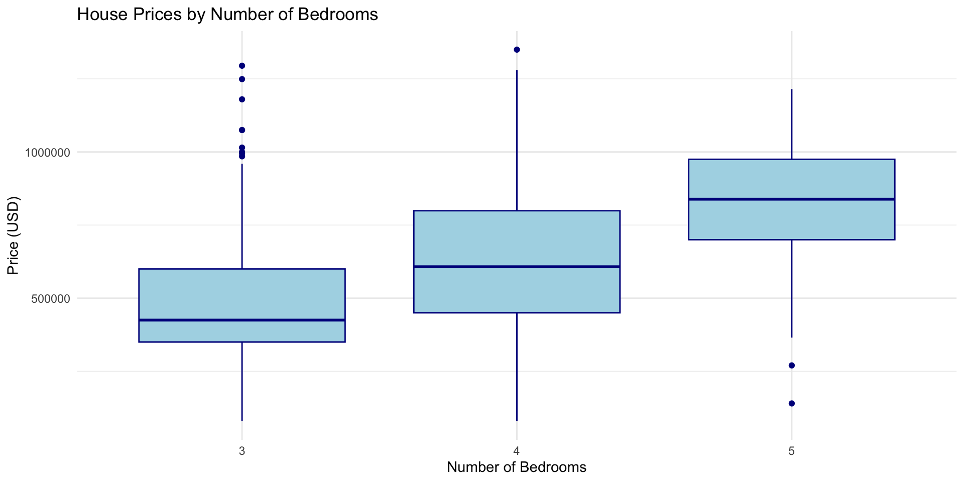
Figure 1: House Prices by Number of Bedrooms

Price vs bedrooms

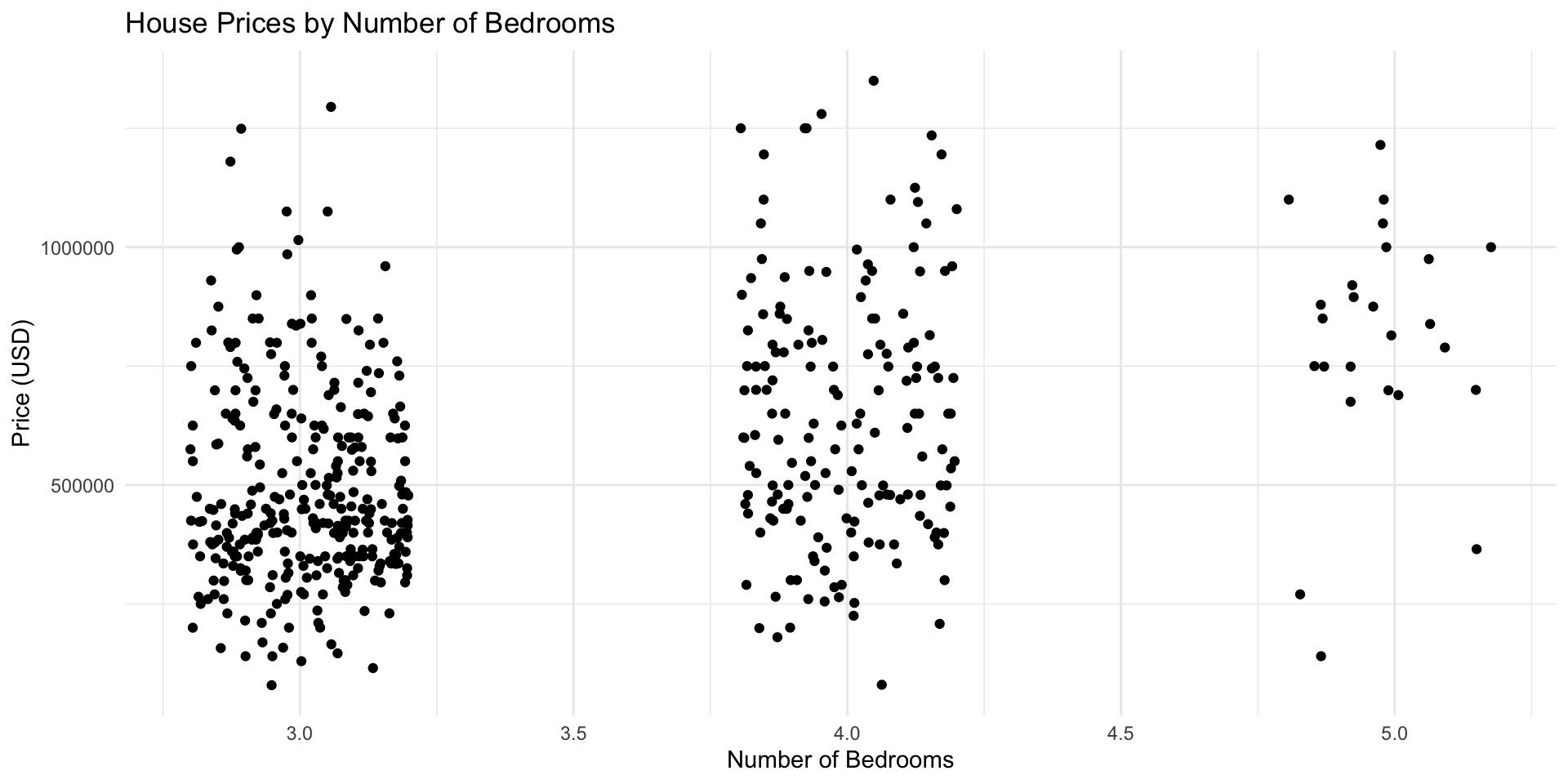
Figure 2: House Prices vs Number of Bedrooms (jittered scatterplot)

Price vs bedrooms

On average, more bedrooms = higher price
Variability among houses with any given number of bedrooms – why?
- Other factors not in the model
- “Random” variation (who is in and out of the market, buyer/seller motivation, etc)

Price vs bedrooms

Looks like the relationship is close to linear
- What does that mean?
- The average price difference between 2 and 3 bedroom houses is about the same as 3 vs 4
Let’s fit a linear regression model to quantify the relationship: \[ \widehat{\text{price}} = \hat\beta_0 + \hat\beta_1 \times \text{beds} \]

Price vs bedrooms

model_bed <- lm(price ~ beds, data = houses)
summary(model_bed)


Call:
lm(formula = price ~ beds, data = houses)

Residuals:
    Min      1Q  Median      3Q     Max 
-657616 -151806  -46830  138220  808220 

Coefficients:
            Estimate Std. Error t value            Pr(>|t|)    
(Intercept)    20527      60308  0.3404              0.7337    
beds          155418      17355  8.9551 <0.0000000000000002 ***
---
Signif. codes:  0 '***' 0.001 '**' 0.01 '*' 0.05 '.' 0.1 ' ' 1

Residual standard error: 229040 on 506 degrees of freedom
Multiple R-squared:  0.1368,    Adjusted R-squared:  0.1351 
F-statistic: 80.193 on 1 and 506 DF,  p-value: < 0.000000000000000222

Reading the regression table

For now, focus on the coefficients:
- Intercept $\hat\beta_0$: $20,527
- Slope $\hat\beta_1$: $155,418
- Fitted line: \[ \widehat{price} = 20,527 + 155,418 \times beds \]

Visualizing the fit

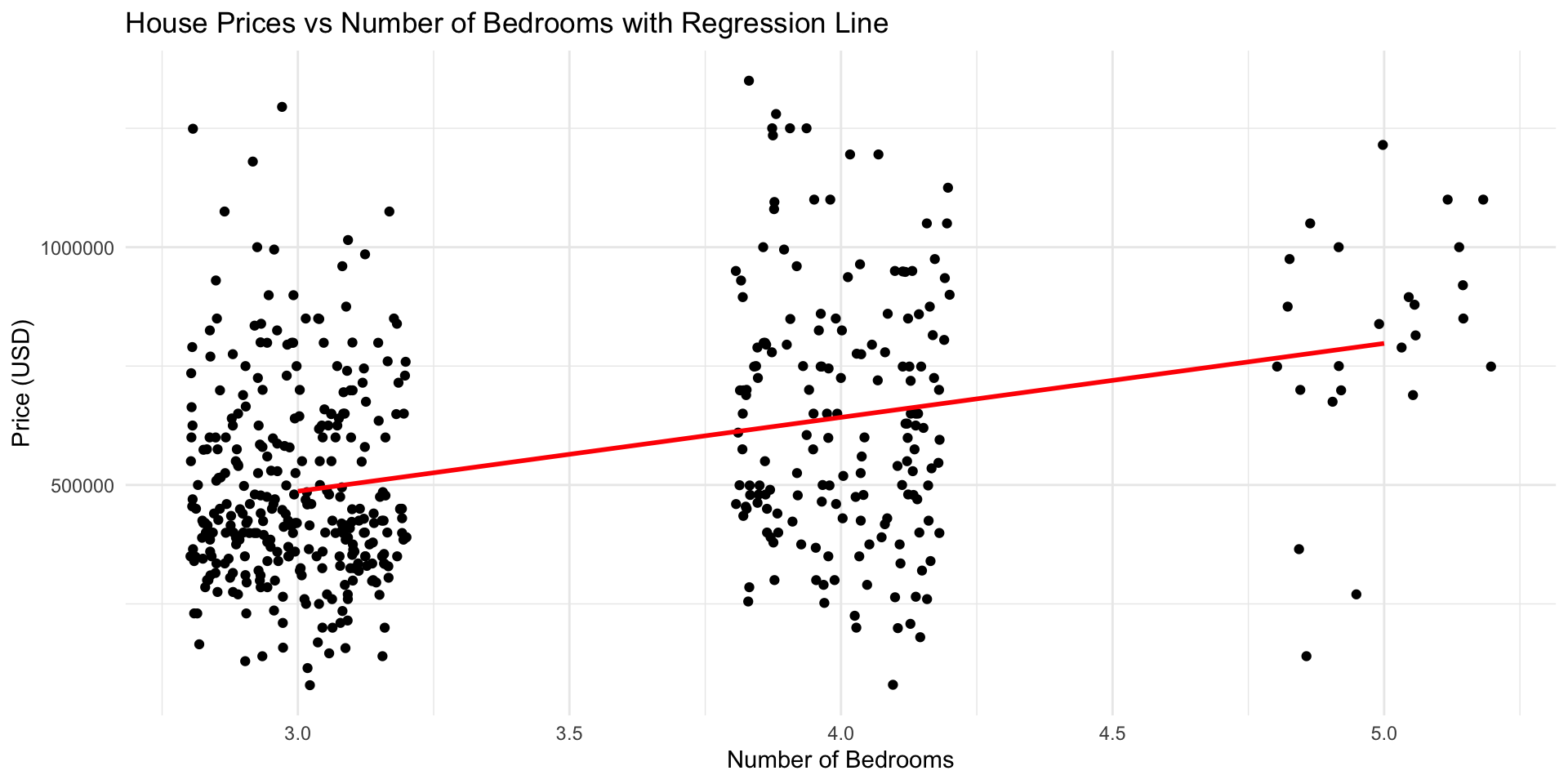
Figure 3: House Prices vs Number of Bedrooms with Regression Line

Price vs living area

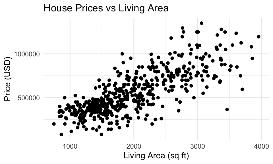
Only three distinct values for bedrooms
Let’s look at a continuous predictor: living area (square feet)

Practice

Find the intercept and slope in the regression output below, and write the equation predicting price from living area

model_area <- lm(price ~ area, data = houses)
summary(model_area)


Call:
lm(formula = price ~ area, data = houses)

Residuals:
    Min      1Q  Median      3Q     Max 
-604840  -90641    2955   83298  519720 

Coefficients:
             Estimate Std. Error t value            Pr(>|t|)    
(Intercept)  4296.668  21017.955  0.2044              0.8381    
area          279.139     10.101 27.6337 <0.0000000000000002 ***
---
Signif. codes:  0 '***' 0.001 '**' 0.01 '*' 0.05 '.' 0.1 ' ' 1

Residual standard error: 155630 on 506 degrees of freedom
Multiple R-squared:  0.60146,   Adjusted R-squared:  0.60067 
F-statistic: 763.62 on 1 and 506 DF,  p-value: < 0.000000000000000222

Practice

Intercept: $\hat\beta_0$: 4297
Slope: $\hat\beta_1$: 279.14
Fitted line: \[ \widehat{\text{price}} = 4297 + 279.14 \times \text{area} \]

Visualizing the fit

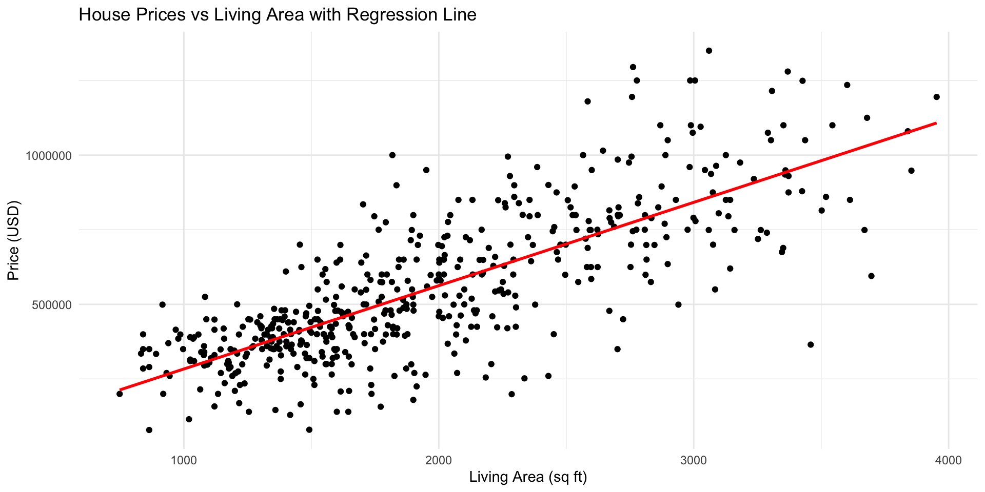
OK who cares?

Linear regression has two basic use cases:

To generate predictions
To understand how changes in the predictors X relate to changes in the actual or predicted outcome Y

Making predictions

Say I want to predict the sale price of a newly listed house with 2,000 sq ft of living area
Using our model, my guess is

\[ \widehat{\text{price}} \approx 4297 + 279.14 \times 2000 = 562577 \]

(Without rounding the intercept/slope we get $562,576)

Making predictions (graphically)

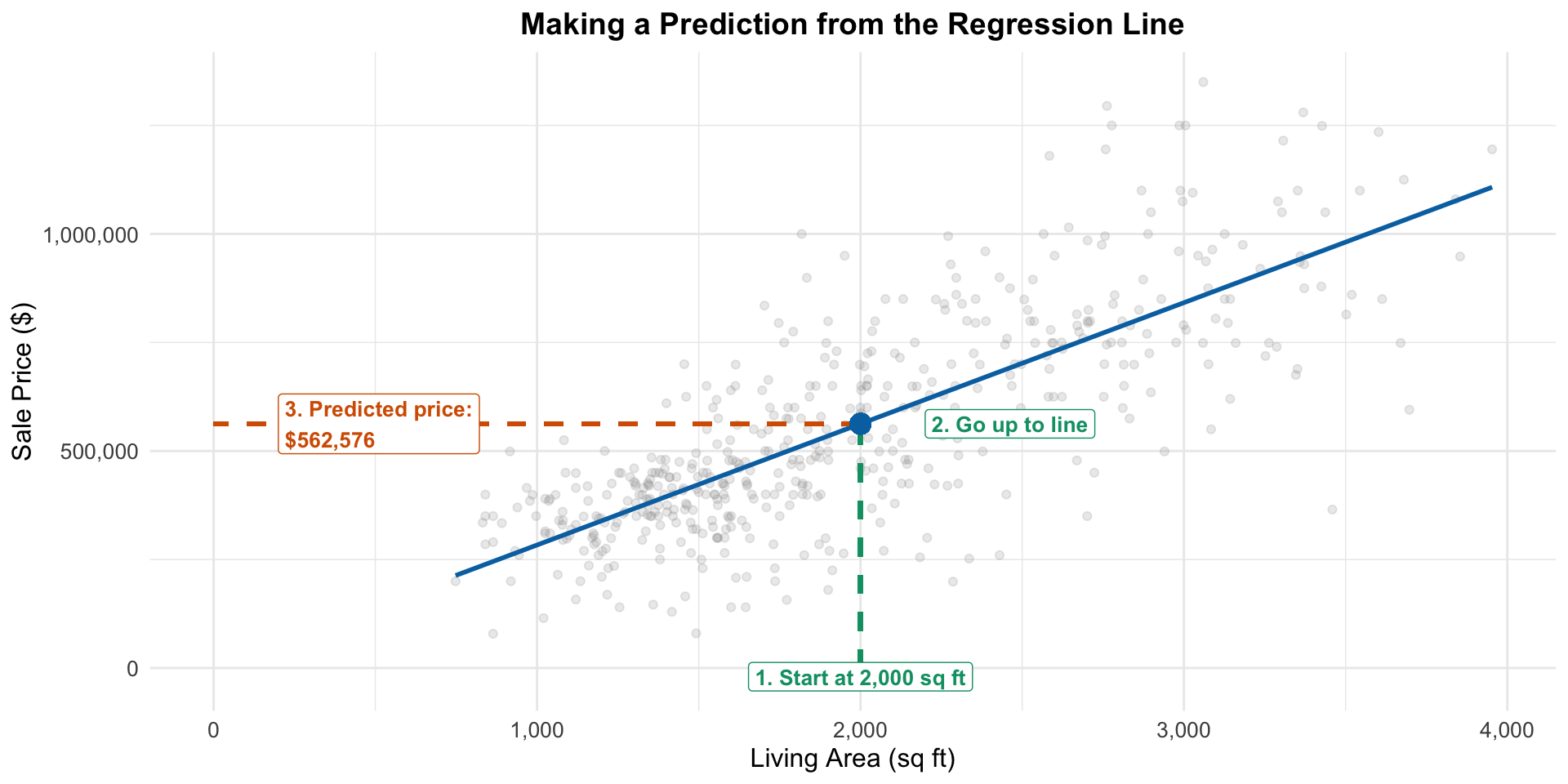
Making predictions

You should know how to do this by hand (read off the linear equation, plug in the x value, calculate the prediction)
That’s how you check your understanding
But in practice, you’ll usually use R to do this for you

new_data <- data.frame(area = 2000)
predicted_price <- predict(model_area, newdata = new_data)
predicted_price

        1 
562575.52

Interpreting the predicted value

The predicted price for a house with 2,000 sq ft of living area is $562,576
- For a newly listed 2,000 sqft house, this is our best guess at the sale price
- It is also the estimated average sale price for all houses with 2,000 sq ft of living area in these three Austin zips
Think about the regression prediction as the model’s estimated average outcome for all similar units (2000 sqft houses)

Summarizing relationships

We can use the fitted model to summarize the relationship between X’s (predictors) and Y (outcome)
The slope tells us how much the predicted outcome (price) changes for a one unit increase in the predictor (area)
- For each additional square foot of living area, the predicted price increases by $279.14
- Comparing two houses that differ in size by one sqft, the larger house has predicted price that is $279.14 higher

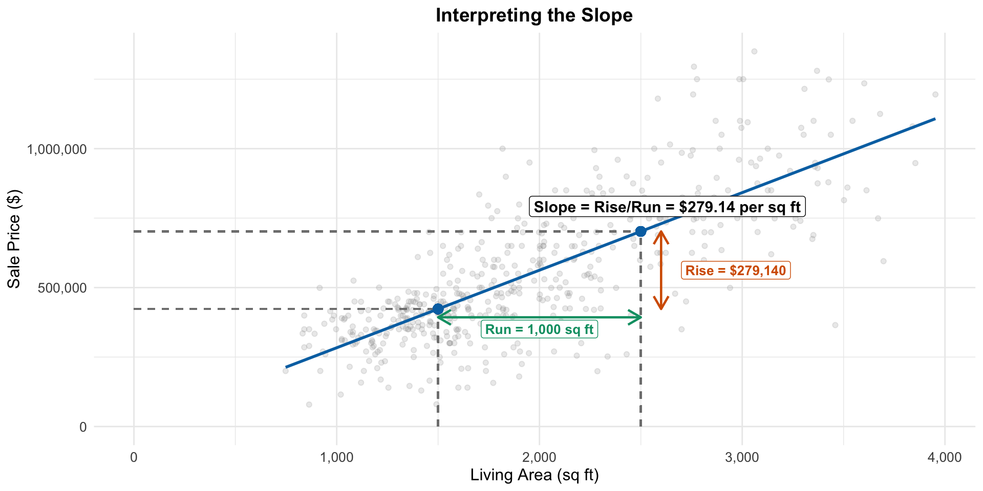
Interpreting the slope

Remember, we can think about the prediction as the (estimated) average outcome for all units with that X value
So the slope also tells us:
- If we compare two houses that differ in size by 1 sqft, the larger house has a predicted value that is $279.14 higher
- On average, houses that are 1 sqft larger sell for $279.14 more

Interpreting the intercept

In general a simple linear regression fit is: \[ \hat Y = \hat \beta_0 + \beta_1 X \]
The intercept $\hat\beta_0$ is the predicted price when $X = 0$ (area = 0 sqft)
- In our case, this is $4,297
Does this make sense, and is it a reliable number?

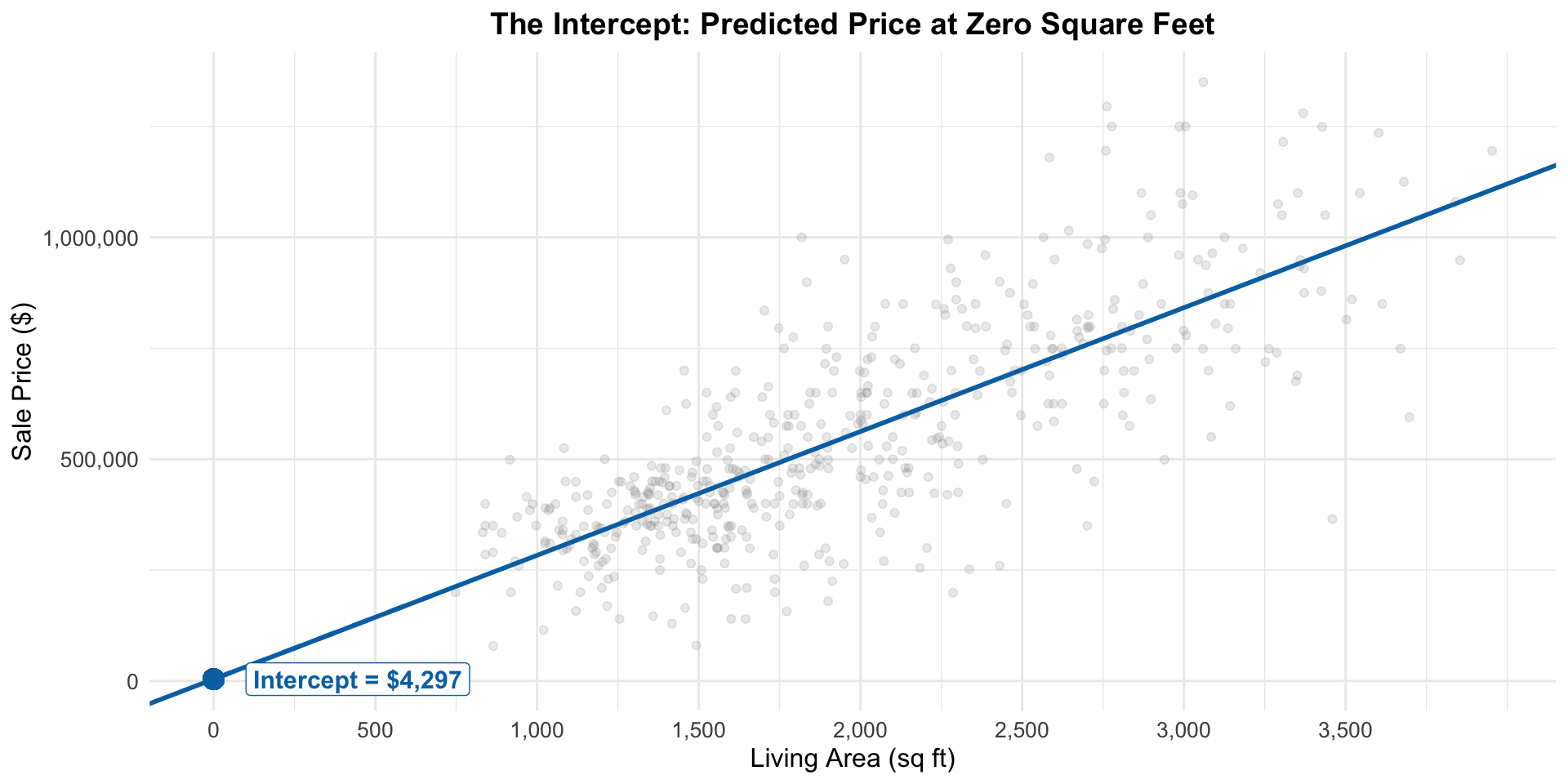
Interpreting the intercept

Does it make sense? Maybe.

No, a house with 0 sq ft doesn’t exist
Yes, we could sell an empty lot

Is it reliable? No.

Our smallest house is about 800 sqft; we have no data on bare lots
Don’t extrapolate far beyond the observed data range

Practice: Price vs beds

Revisit the regression of price on number of bedrooms

Predict the sale price of a house with 3 bedrooms
According to our model, what’s the average sale price of a house with three bedrooms?
What is the interpretation of the slope in that model?
What is the interpretation of the intercept in that model? Is it meaningful?

Multiple regression: Price vs area and beds

So far, we’ve looked at simple linear regression with one predictor.

What if we want to include both living area and number of bedrooms as predictors?

More (useful) information should give us better predictions, right?
What can we learn about relationships between variables?

Multiple regression: Price vs area and beds

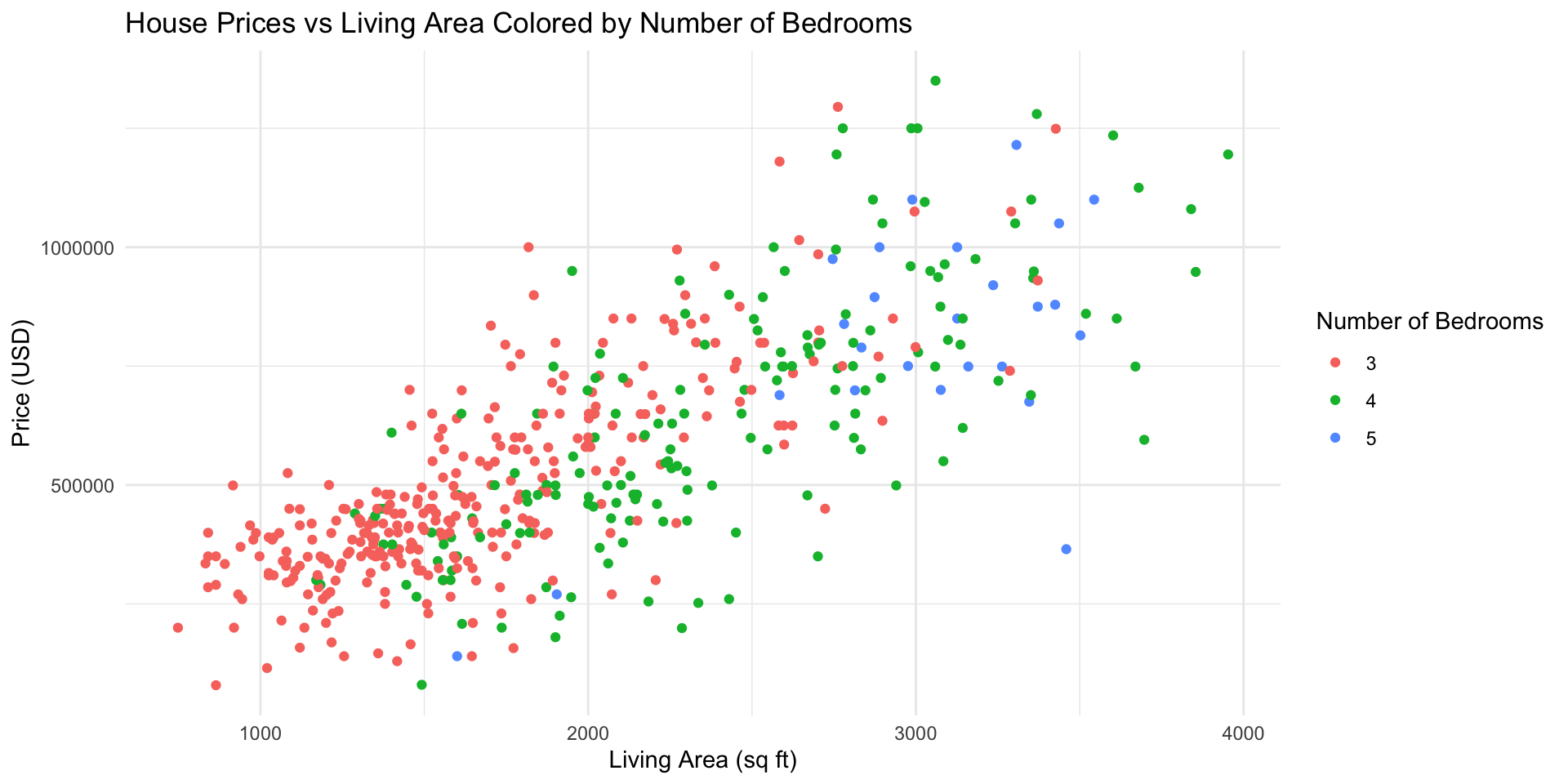
Multiple regression fit

model_multi <- lm(price ~ area + beds, data = houses)
summary(model_multi)


Call:
lm(formula = price ~ area + beds, data = houses)

Residuals:
    Min      1Q  Median      3Q     Max 
-554870  -84304    -988   80190  492369 

Coefficients:
              Estimate Std. Error t value              Pr(>|t|)    
(Intercept) 153643.148  40647.355  3.7799             0.0001756 ***
area           310.813     12.401 25.0639 < 0.00000000000000022 ***
beds        -61774.861  14477.102 -4.2671            0.00002366 ***
---
Signif. codes:  0 '***' 0.001 '**' 0.01 '*' 0.05 '.' 0.1 ' ' 1

Residual standard error: 153050 on 505 degrees of freedom
Multiple R-squared:  0.61533,   Adjusted R-squared:  0.6138 
F-statistic:  403.9 on 2 and 505 DF,  p-value: < 0.000000000000000222

Multiple regression fit

From the table, the regression fit (prediction equation) is: \[ \widehat{\text{price}} = 153643 + 310.81 \times \text{area} -61775 \times \text{beds} \]

310.81 is the coefficient for area (dollars per sqft)
-61774.86 is the coefficient for beds (dollars per bedroom)

Multiple regression predictions

We can make predictions just like before: Plug in X’s and get predicted Y’s
In R:

new_data1 <- data.frame(area = 2000, beds = 4)
predict(model_multi, newdata = new_data1)

        1 
528169.15

Check by hand to make sure you understand!

Interpreting the regression fit

We’ve seen three regression fits so far:

\[ \widehat{\text{price}} = 20527 + 155418 \times \text{beds} \]

\[ \widehat{\text{price}} = 4297 + 279.14 \times \text{area} \]

\[ \widehat{\text{price}} = 153643 + 310.81 \times \text{area} -61775 \times \text{beds} \]

How do the two simple regression slopes compare to the corresponding multiple regression coefficients?

Area’s got bigger
Beds’ got smaller and changed sign
Why???

How do we interpret the coefficients?

Intercept: Prediction when all X’s are 0 – a house with no beds and no area
The coefficients on our two variables are similar to slopes, with one important difference.
Bedrooms coefficient ($-61775):
- For a one bedroom increase, holding area constant, the predicted price decreases by $61775

What does “holding area constant” mean?

If we have two houses with identical areas that differ by 1 bedroom, the one with the extra bedroom has a predicted sale price $61775 lower
When we compare two houses of the same size, on average, the one with more bedrooms sells for less! (a decrease of $61775 per bed)
The MLR coefficients represent adjusted comparisons – we are comparing houses that differ in one predictor (beds) but are identical in all other predictors in the model (area)

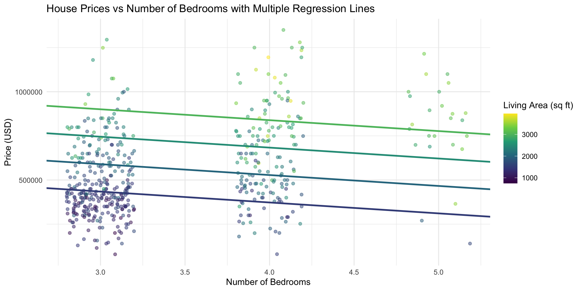
One multiple regression is many simple regressions

We can think about the multiple regression as defining a different simple regression predicting price from beds for any given area.

The equation for that line is:

\[ \widehat{\text{price}} = \underbrace{[153643 + 310.81 \times \text{area}]}_{\text{area specific intercept}} \underbrace{-61775}_{\text{common slope}} \times \text{beds} \]

How do we interpret the coefficients?

For example:

For a house with 1,500 sqft: \[\begin{align} \widehat{\text{price}} &= [ 153643 + 310.81 \times 1500 ] -61775 \times \text{beds}\\ &= 619858 -61775 \times \text{beds} \end{align}\]
For a house with 2,000 sqft: \[\begin{align} \widehat{\text{price}} &= [ 153643 + 310.81 \times 2000 ] -61775 \times \text{beds}\\ &= 775263 -61775 \times \text{beds} \end{align}\]

Visualizing the model fit

Does the MLR estimate make sense?

In our model, if we compare two houses of the same size, the one with more bedrooms has a lower predicted price.

Does this make sense?

If the area is the same, then a house with more bedrooms has smaller rooms overall
If we can’t add area to the house, how do we get another bedroom?
- Cut the living room in half?
- Split a bedroom?
- Do any of these add value?

Is it consistent with the data?

Let’s do a simple exercise: Compare the average sale price for 3 and 4 bed houses of similar sizes

We don’t have enough data on houses of any single size to compare historical prices (this is one reason to fit a model!)
But if our story is true, when we look at subsets of houses with similar sizes, we should see lower average prices for 4 bed vs 3 bed houses

Returning to the data

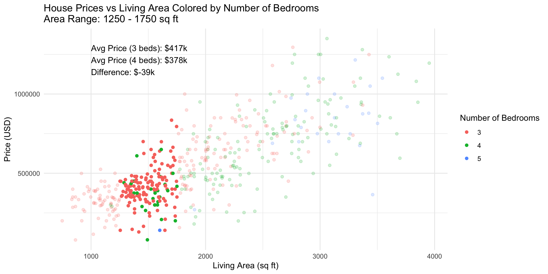
Figure 4: Area Range: 1250-1750 sq ft

Returning to the data

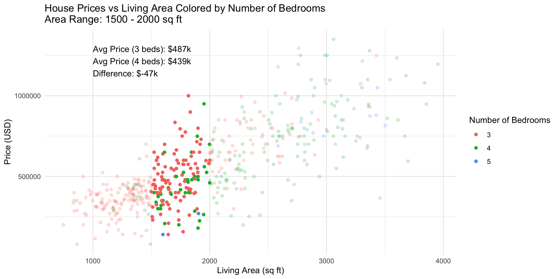
Figure 5: Area Range: 1500-2000 sq ft

Returning to the data

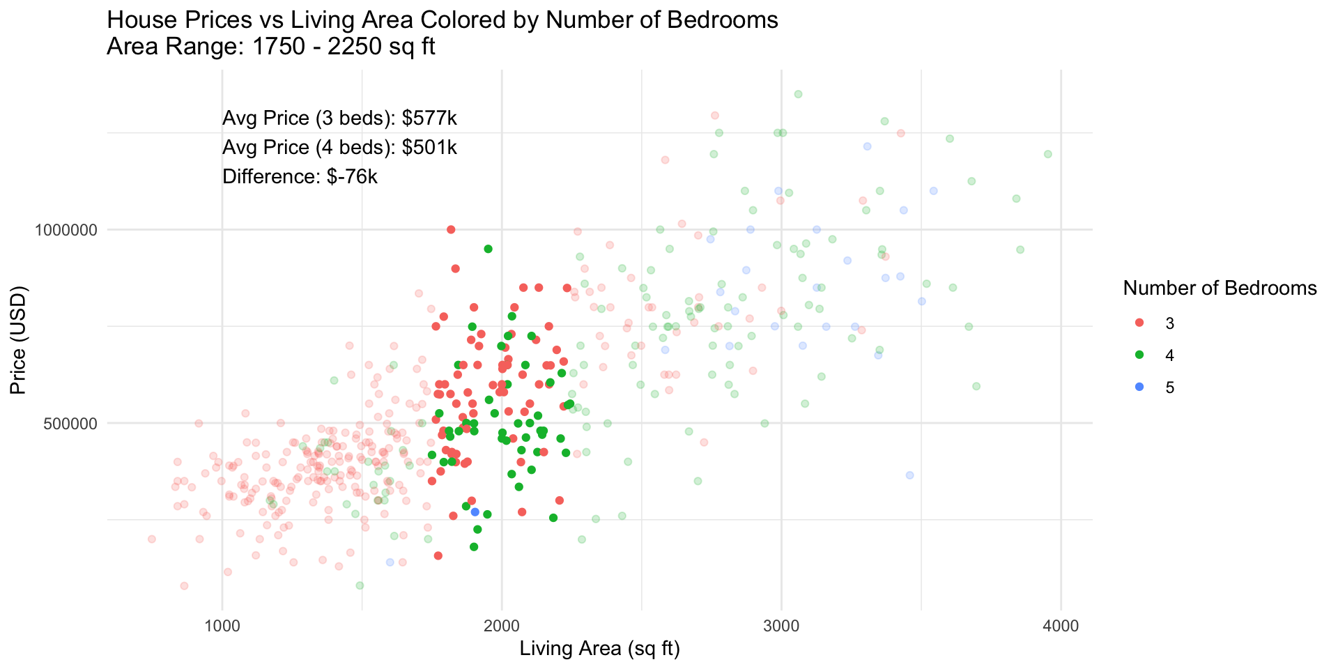
Figure 6: Area Range: 1750-2250 sq ft

Returning to the data

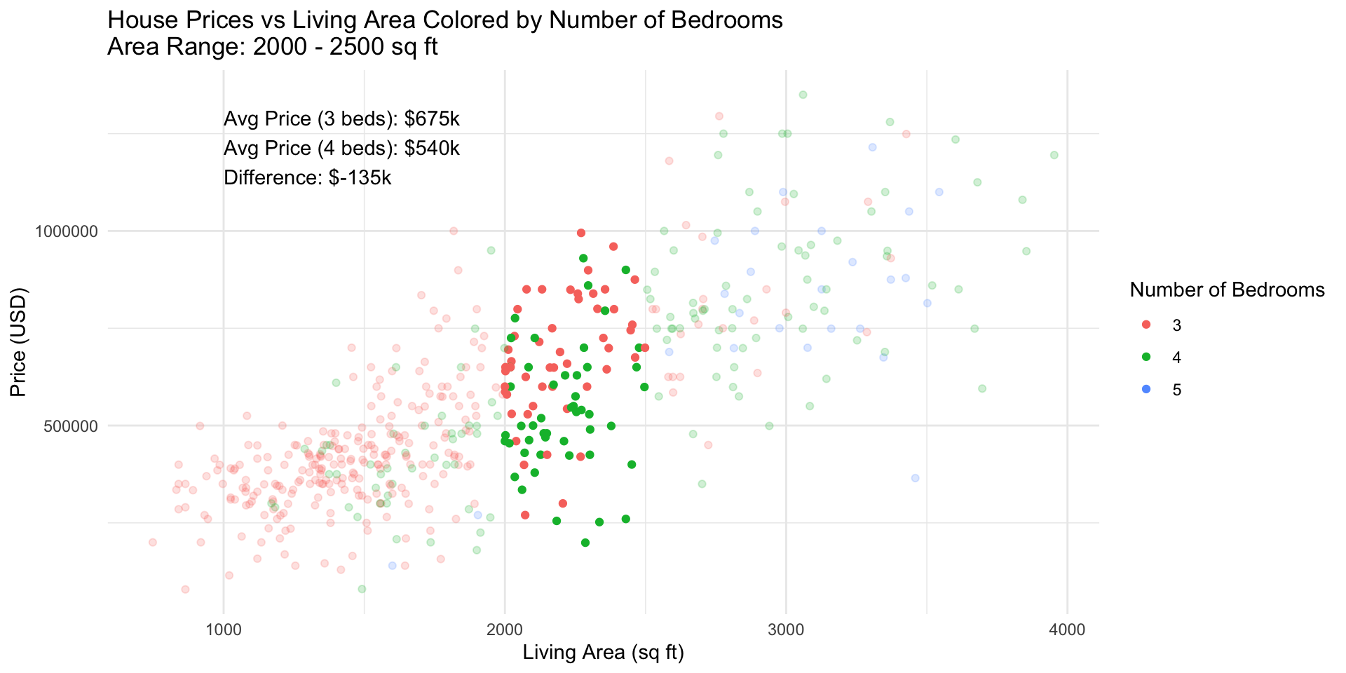
Figure 7: Area Range: 2000-2500 sq ft

Returning to the data

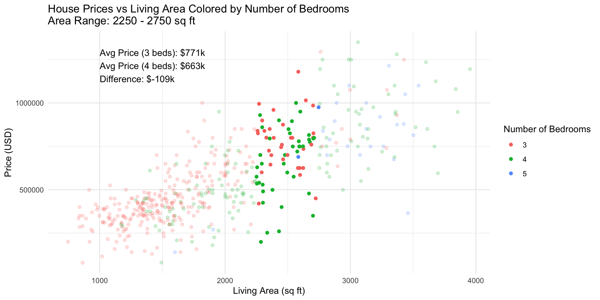
Figure 8: Area Range: 2250-2750 sq ft

What’s going on?

Larger houses tend to have more bedrooms (area and beds are correlated)
Both predict sale prices
Without area in the model, beds is a proxy for size:
- More beds = larger house = higher price on average
- This gives us the positive association/slope in the model with just beds

Which model is “right”?

They both are! They just estimate different things:

Simple regression: The overall linear relationship between beds and price, irrespective of size
Multiple regression: The linear relationship between beds and price when we compare houses of the same size

Multiple regression “adjusts” or “controls” for size, by comparing like vs like.

Interpreting the area coefficient

In the multiple regression of price on area and beds, the coefficient for area is 310.81 dollars per sq ft
Comparing two houses with the same number of bedrooms that differ in size by 1 sqft, the larger house has a predicted price that is $310.81 higher
On average, among all houses with the same number of bedrooms, larger houses sell for more and the difference is about $310.81 per additional sqft

What’s going on with the area coefficient?

In the simple regression of price on area, the coefficient is 279.14 dollars per sq ft
In the multiple regression of price on area and beds, the coefficient is 310.81 dollars per sq ft
Why did it go up?

Revisiting the data

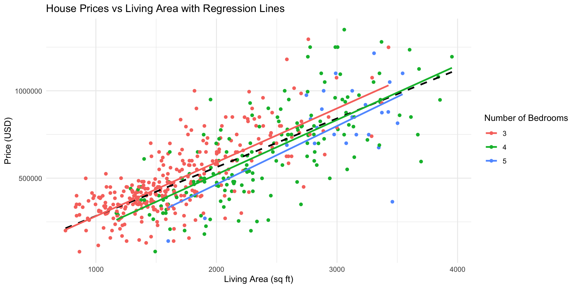
When we only compare houses of the same number of bedrooms, we do indeed get steeper slopes than the overall regression line (in black)!

What’s going on with the area coefficient?

In the simple regression of price on area, the coefficient is 279.14 dollars per sq ft
In the multiple regression of price on area and beds, the coefficient is 310.81 dollars per sq ft
Why did it go up? Without beds in the model, area was partially capturing the effect of beds!

Example 2

What personal characteristics about an instructor do you think are predictive of the scores they receive on student evaluations?

Hamermesh & Parker (2005) data set

Student evaluations of $N=463$ instructors at UT Austin, 2000-2002
For each instructor:
- eval: average student evaluation of teacher
- beauty: average beauty score from a six-student panel (z-score, 0 is average)
- gender: male or female
- credits: single- or multi-credit course
- age: age of instructor
- (and more…)

Explore the data: `eval`

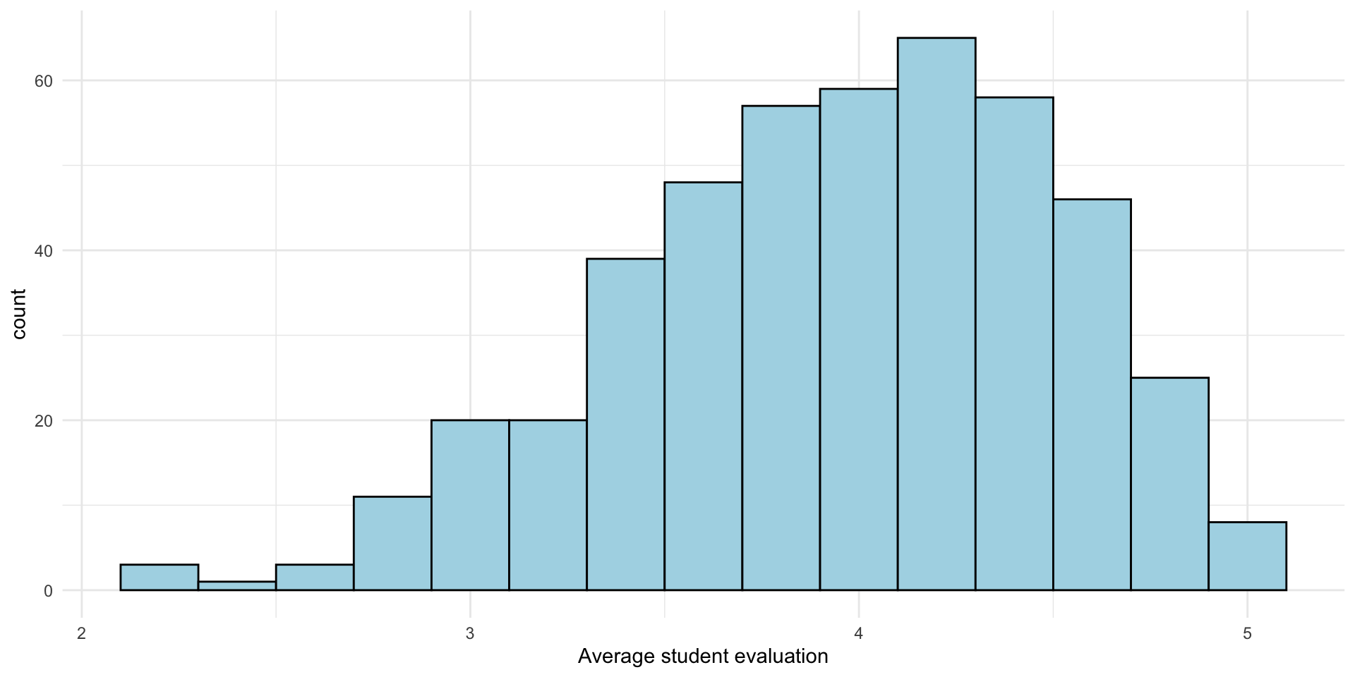
Explore the data: `beauty`

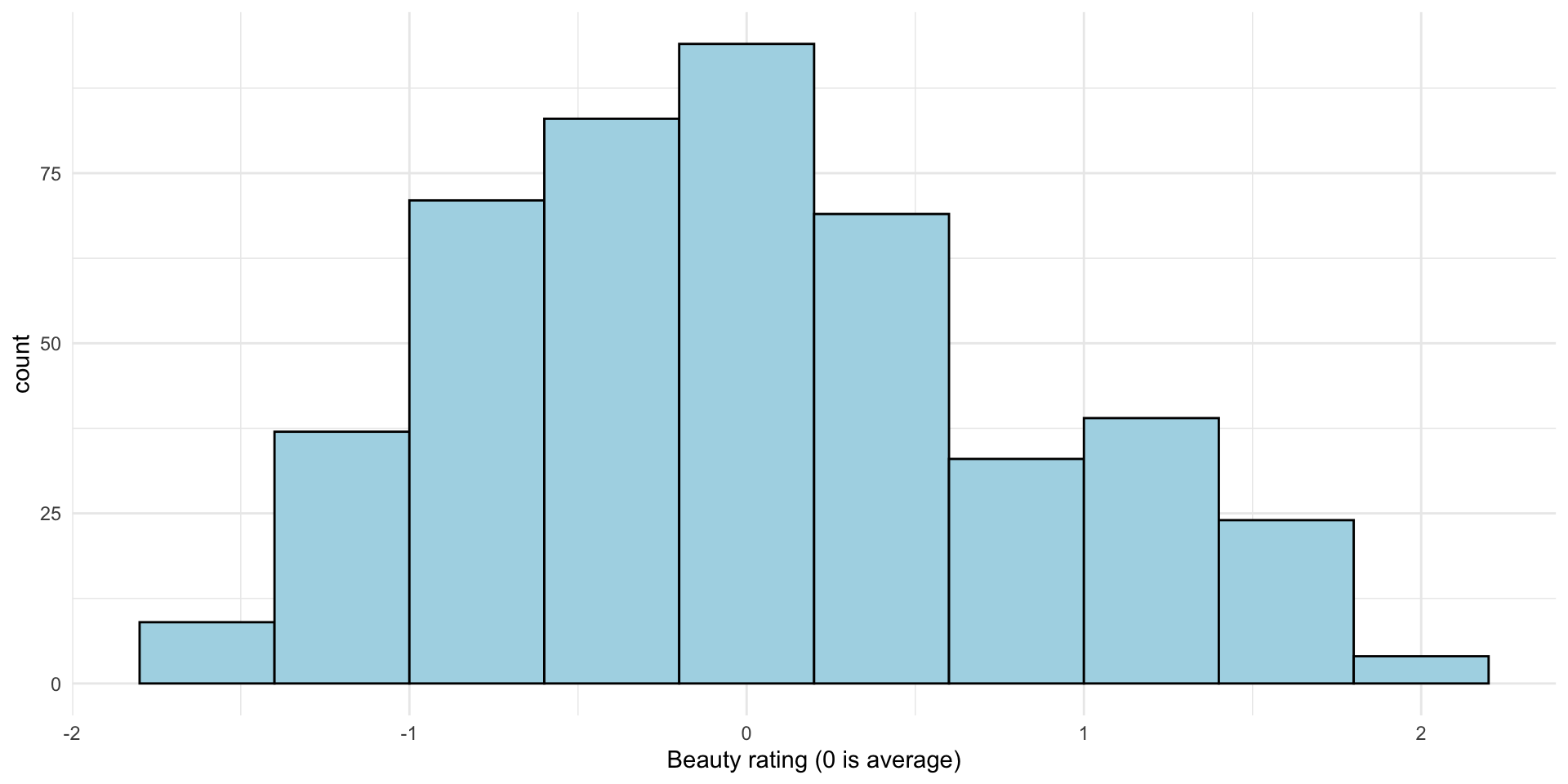
Do you think there is a positive or negative relationship between beauty and evaluations?

Explore the data

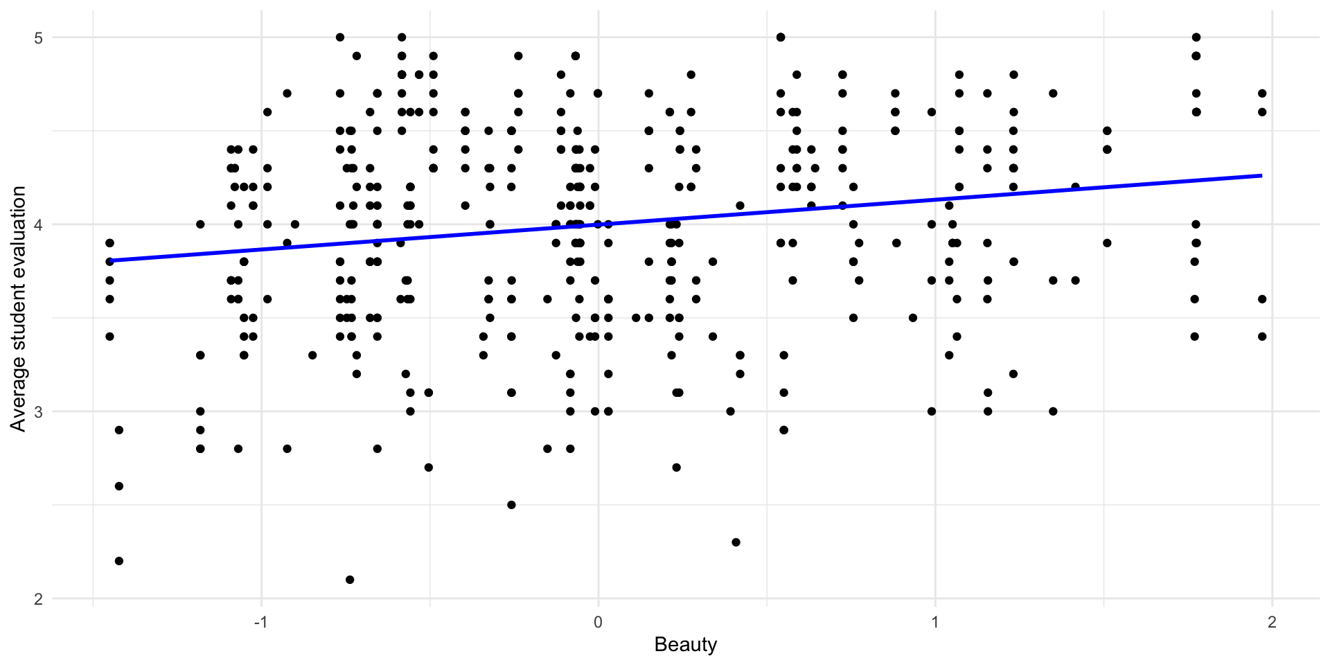
The simple regression fit


Call:
lm(formula = eval ~ beauty, data = profs)

Residuals:
    Min      1Q  Median      3Q     Max 
-1.8002 -0.3630  0.0725  0.4021  1.1037 

Coefficients:
            Estimate Std. Error t value             Pr(>|t|)    
(Intercept)   3.9983     0.0253  157.73 < 0.0000000000000002 ***
beauty        0.1330     0.0322    4.13             0.000042 ***
---
Signif. codes:  0 '***' 0.001 '**' 0.01 '*' 0.05 '.' 0.1 ' ' 1

Residual standard error: 0.545 on 461 degrees of freedom
Multiple R-squared:  0.0357,    Adjusted R-squared:  0.0336 
F-statistic: 17.1 on 1 and 461 DF,  p-value: 0.0000425

Interpreting the intercept

Intercept:

When beauty = 0 (average), predicted eval = 3.998 points
The average evaluation for an average-looking instructor
Meaningful this time!

Interpreting the slope

Slope:

For a one unit (standard deviation) increase in beauty, the predicted eval increases by 0.13 points
Comparing two instructors who differ by 1 SD on beauty, on average the more attractive instructor has an eval score 0.13 points higher

Is this the whole story?

Probably not!

Lots of other predictors to consider – could the positive association be due to another variable that isn’t in the model yet (think bedrooms and living area)?
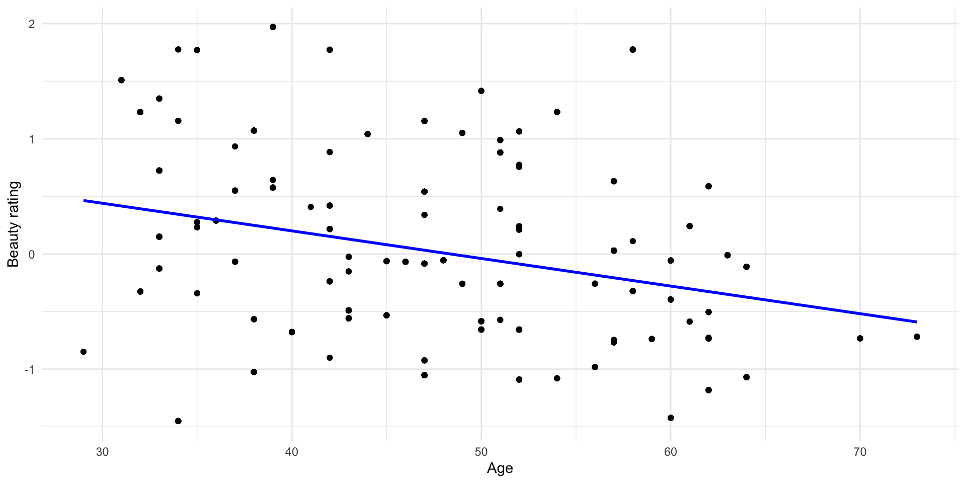
Age might be important here – how?
- On average, older instructors are probably less hot
- As they age instructors might get better at teaching (experience) – or worse (stale or out of touch)

Is age actually correlated with beauty?

Multiple regression: eval on beauty and age

model_beauty <- 
    lm(eval ~ beauty, data = profs)
summary(model_beauty)


Call:
lm(formula = eval ~ beauty, data = profs)

Residuals:
    Min      1Q  Median      3Q     Max 
-1.8002 -0.3630  0.0725  0.4021  1.1037 

Coefficients:
            Estimate Std. Error t value             Pr(>|t|)    
(Intercept)   3.9983     0.0253  157.73 < 0.0000000000000002 ***
beauty        0.1330     0.0322    4.13             0.000042 ***
---
Signif. codes:  0 '***' 0.001 '**' 0.01 '*' 0.05 '.' 0.1 ' ' 1

Residual standard error: 0.545 on 461 degrees of freedom
Multiple R-squared:  0.0357,    Adjusted R-squared:  0.0336 
F-statistic: 17.1 on 1 and 461 DF,  p-value: 0.0000425

model_beauty_age <- 
    lm(eval ~ beauty + age, data = profs)
summary(model_beauty_age)


Call:
lm(formula = eval ~ beauty + age, data = profs)

Residuals:
    Min      1Q  Median      3Q     Max 
-1.8024 -0.3651  0.0741  0.3991  1.1021 

Coefficients:
            Estimate Std. Error t value             Pr(>|t|)    
(Intercept) 3.984401   0.133730   29.79 < 0.0000000000000002 ***
beauty      0.134063   0.033744    3.97             0.000082 ***
age         0.000287   0.002715    0.11                 0.92    
---
Signif. codes:  0 '***' 0.001 '**' 0.01 '*' 0.05 '.' 0.1 ' ' 1

Residual standard error: 0.546 on 460 degrees of freedom
Multiple R-squared:  0.0358,    Adjusted R-squared:  0.0316 
F-statistic: 8.53 on 2 and 460 DF,  p-value: 0.00023

Interpreting the coefficients

In this case, whether we compare instructors of the same age or not, we get the same answer: Hotter instructors get higher evaluations on average.
Good(ish) news – we ruled out one alternative explanation for the association between beauty and eval
Are there others?

Summary

As we add or remove variables in regression models, the coefficients on other variables can go up, down, or stay about the same
It all depends on the relationships
1. Among the predictors
2. Between the predictors and the outcome

If we want to interpret our models, we need to think carefully about how we specify them.

Summary

In this course we’ll learn how to build models that

Estimate the effects we want
Make the best possible predictions

These are not always the same!

Next time: Errors and uncertainty

The missing part of the story so far is estimation/prediction error and uncertainty. For example:

Does the association between beauty and evals hold among ALL instructors, or just in this sample?
- Could we be looking at a chance association that would disappear if we could get data on everyone?

Next time: Errors and uncertainty

The missing part of the story so far is estimation/prediction error and uncertainty. For example:

How accurately can we predict the sale price of a house from its size and other factors?
- How do we quantify prediction errors? Even with many variables our predictions will be off by some amount. How wrong should we expect to be?

Intro and Linear Regression Refresher

Introduction to the course

Canvas

Class structure

Grading

Pre-class prep

Pre-class prep

Class Participation

Homework

Checkpoint Quizzes

Mastery Exams

Statistical computing

Getting help

Linear Regression Refresher

Data description:

Price vs bedrooms

Price vs bedrooms

Price vs bedrooms

Price vs bedrooms

Price vs bedrooms

Reading the regression table

Visualizing the fit

Price vs living area

Practice

Practice

Visualizing the fit

OK who cares?

Making predictions

Making predictions (graphically)

Making predictions

Interpreting the predicted value

Summarizing relationships

Interpreting the slope

Interpreting the slope

Interpreting the intercept

Interpreting the intercept

Interpreting the intercept

Practice: Price vs beds

Multiple regression: Price vs area and beds

Multiple regression: Price vs area and beds

Multiple regression fit

Multiple regression fit

Multiple regression predictions

Interpreting the regression fit

How do we interpret the coefficients?

What does “holding area constant” mean?

One multiple regression is many simple regressions

How do we interpret the coefficients?

Visualizing the model fit

Does the MLR estimate make sense?

Is it consistent with the data?

Returning to the data

Returning to the data

Returning to the data

Returning to the data

Returning to the data

What’s going on?

Which model is “right”?

Interpreting the area coefficient

What’s going on with the area coefficient?

Revisiting the data

What’s going on with the area coefficient?

Example 2

Hamermesh & Parker (2005) data set

Explore the data: eval

Explore the data: beauty

Explore the data

The simple regression fit

Interpreting the intercept

Interpreting the slope

Is this the whole story?

Is age actually correlated with beauty?

Multiple regression: eval on beauty and age

Interpreting the coefficients

Summary

Summary

Next time: Errors and uncertainty

Next time: Errors and uncertainty

Explore the data: `eval`

Explore the data: `beauty`