Simple Linear Regression

Linear regression

Linear regression helps us answer questions like:

How does house price change with living area?
Can we predict sales based on advertising spend?
What’s the relationship between study time and exam scores?

Austin home sales

We’ll explore linear regression using data on 508 home sales in Austin, Texas

The data

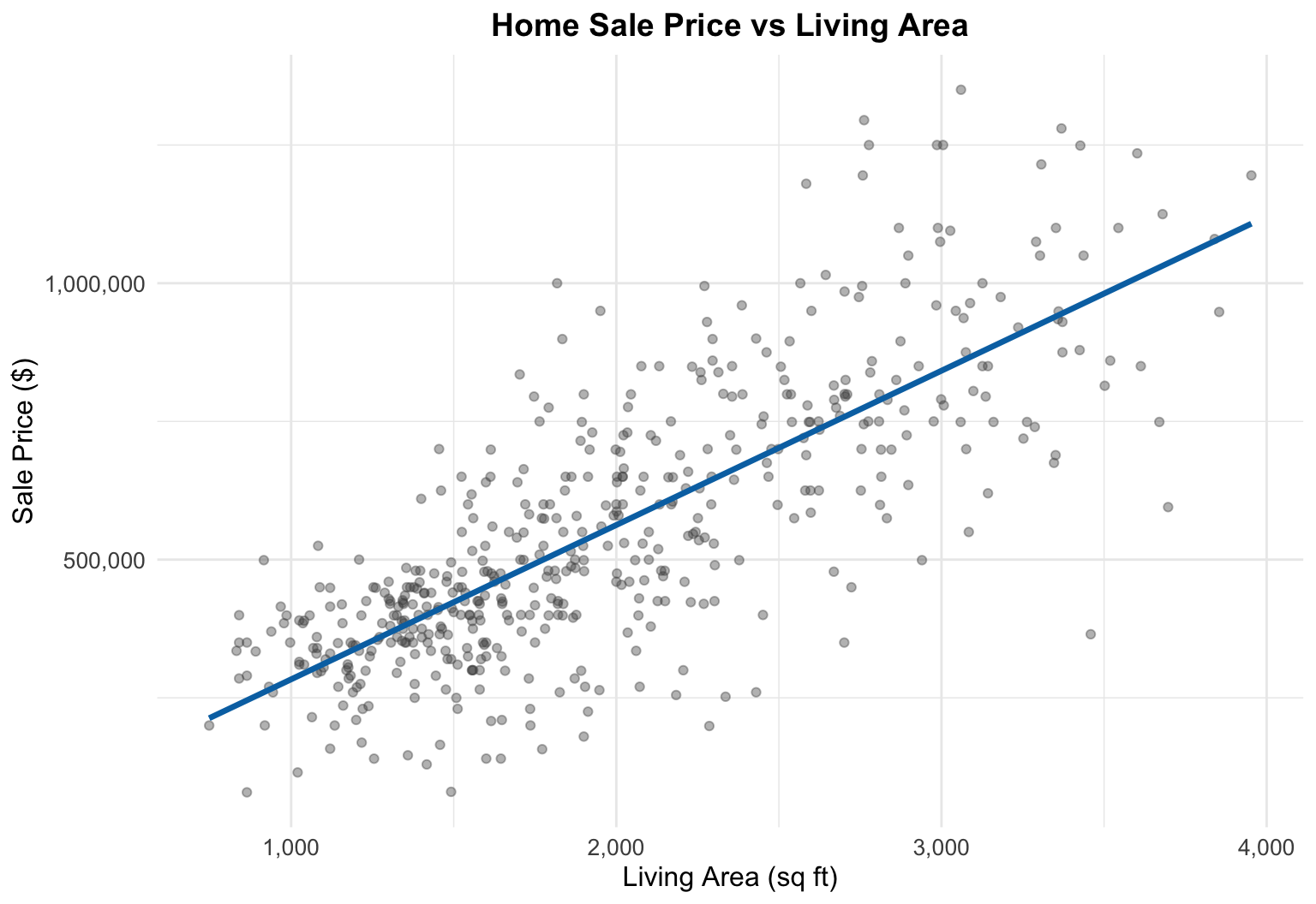
A linear relationship

Clear positive relationship: larger homes tend to sell for more money.
Close to linear—the straight line goes right through the “bulk” of the data, and points look randomly distributed around the line

The fitted line

The line of best fit to the data is given by

\[\widehat{y} = 4297 + 279.14 \times \text{area}\]

“Hats” ($\widehat{~}$) denote estimated or predicted values
$\hat y$ is the predicted price for a house of a given area.
This equation is estimated from data; before we see how we need some additional definitions

Parameters of the line

The equation for the line is determined by two parameter estimates:

$\hat \beta_0 = 4,297$ is the estimated intercept, the predicted price when area equals zero (dollars)
$\hat \beta_1 = 279.14$ is the estimated slope, the predicted change in price for each additional square foot of living area (dollars per sqft)

Fitted values and residuals

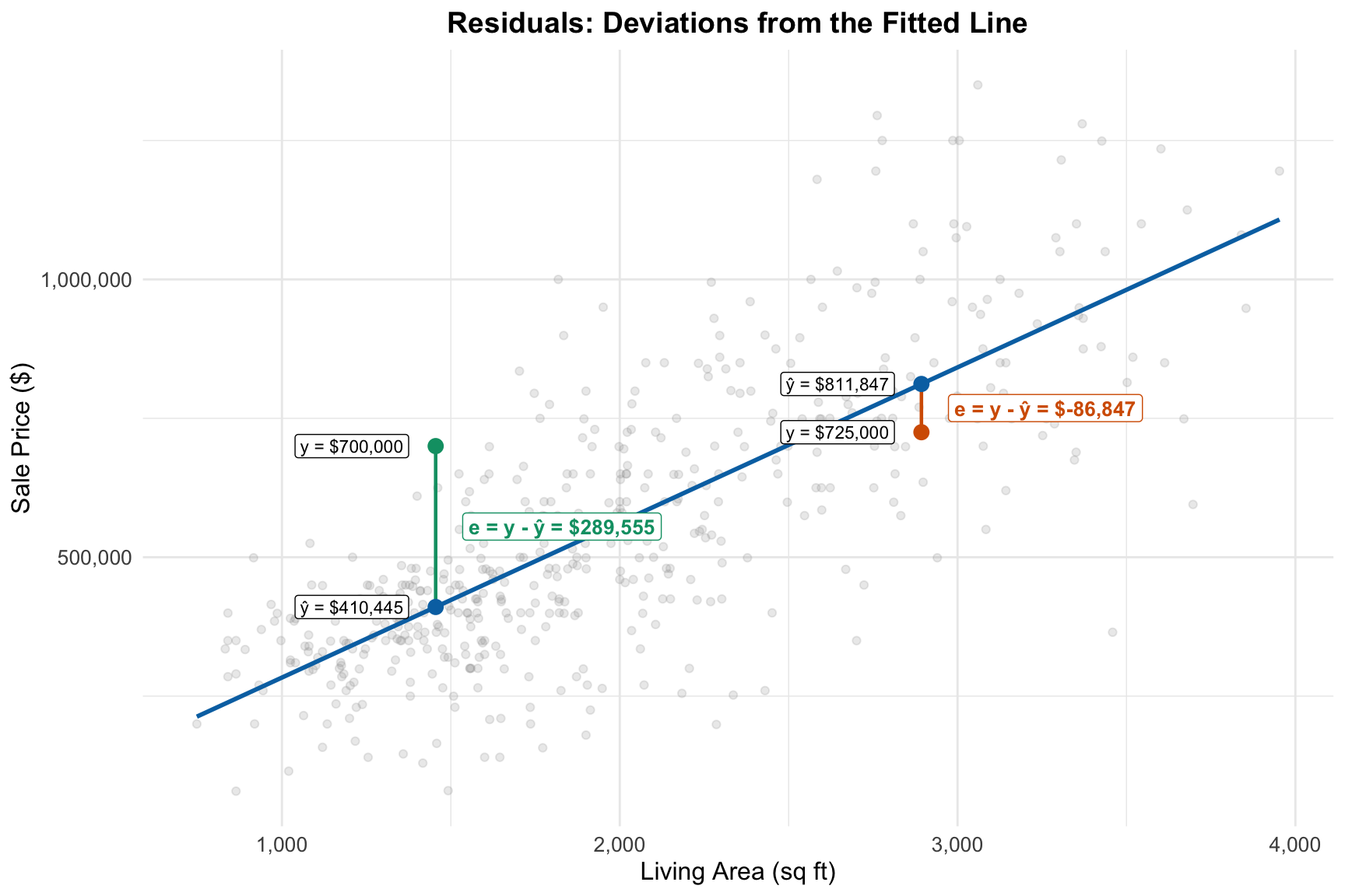
Predictions and prediction errors have special names when computed for the observed $(y_i, x_i)$ pairs:

Predictions: fitted values $\hat y_i = \hat\beta_0+\hat\beta_1x_i$
Prediction errors: residuals $e_i = y_i - \hat y_i$
Each observation can be written \[ y_i = \underbrace{\hat y_i}_{\text{predictable using the model}} + \underbrace{e_i}_\text{unpredictable using the model}} \]

Visualizing fitted values and residuals

Fitting the linear model

OK, so how did we come up with the linear equation?
Find the line that minimizes the average squared prediction error (residual)s over the observed dataset: minimize \[ \frac{1}{n} \sum_{i=1}^{n} e_i^2 = \frac{1}{n}\sum_{i=1}^{n} (y_i - (b_0 + b_1x_i))^2\]
The answer is $b_0 = \hat\beta_0 = 4297$ and $b_1 = \hat \beta_1 = 279.14$
Software will do this for us

The regression model

We think of the data as coming from a population model: \[y_i = \beta_0 + \beta_1 x_i + \epsilon_i\]

where:

$\beta_0$ and $\beta_1$ are unknown population parameters
$\epsilon_i$ represents random variation around the line

Applications of linear regression

Three main uses:

Summarizing trends: What is the nature of the relationship between $x$ and $y$?
Prediction: What value of $y$ should we expect for a given value of $x$?
Quantifying the strength of the linear relationship: How strong is the linear relationship? How much does using $x$ improve our predictions?
Adjusted comparisons: Apples-to-apples comparisons of observations with different $x$ values

Use 1: Summarizing trends

One of the most common uses of linear regression is to summarize the relationship between two variables using the slope and intercept.
These parameters tell us about the nature of the association between the two variables.

Visualizing the slope

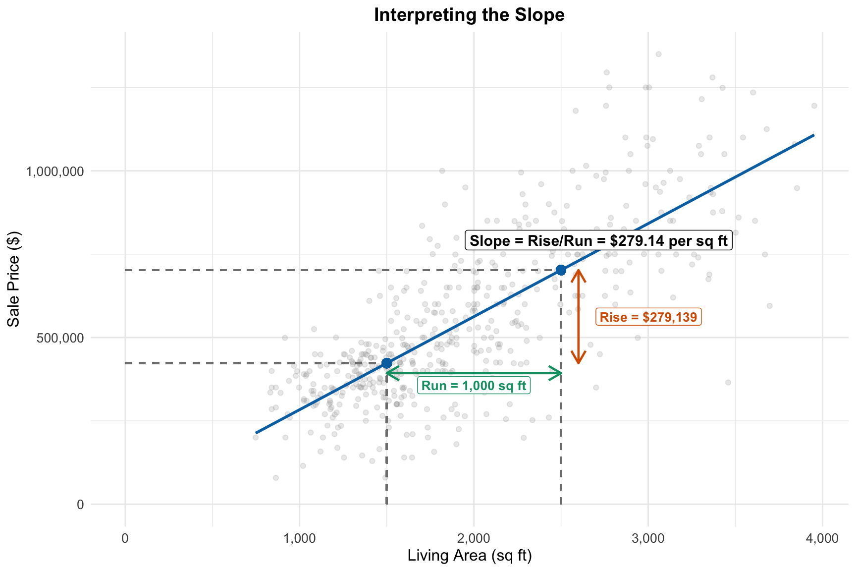
Rise over run

The slope is the “rise over run”—the change in predicted price divided by the change in area.
Comparing a 1,500 sq ft home to a 2,500 sq ft home (an increase of 1,000 sq ft), we predict the price will increase by $279,139.

Interpreting the slope

The slope $\hat\beta_1 = 279.14$ tells us that for each additional square foot of living area, we expect/predict house prices to increase by about $279.14.

Interpreting the slope

Alternatively:

For each additional sqft, the predicted price increases by about $279.14
If we compared two houses which differ in size by one square foot, the larger house would have a predicted sale price that’s $279.14$ higher.
If we compared many houses which differ in size by one square foot, on average the larger houses would sell for $279.14$ more.
One sqft is an arbitrary increment, we could also say something like:
- If we compared two houses which differ in size by 100 sqft, the larger house would have a predicted sale price that’s $27914$ higher.

Interpreting the intercept

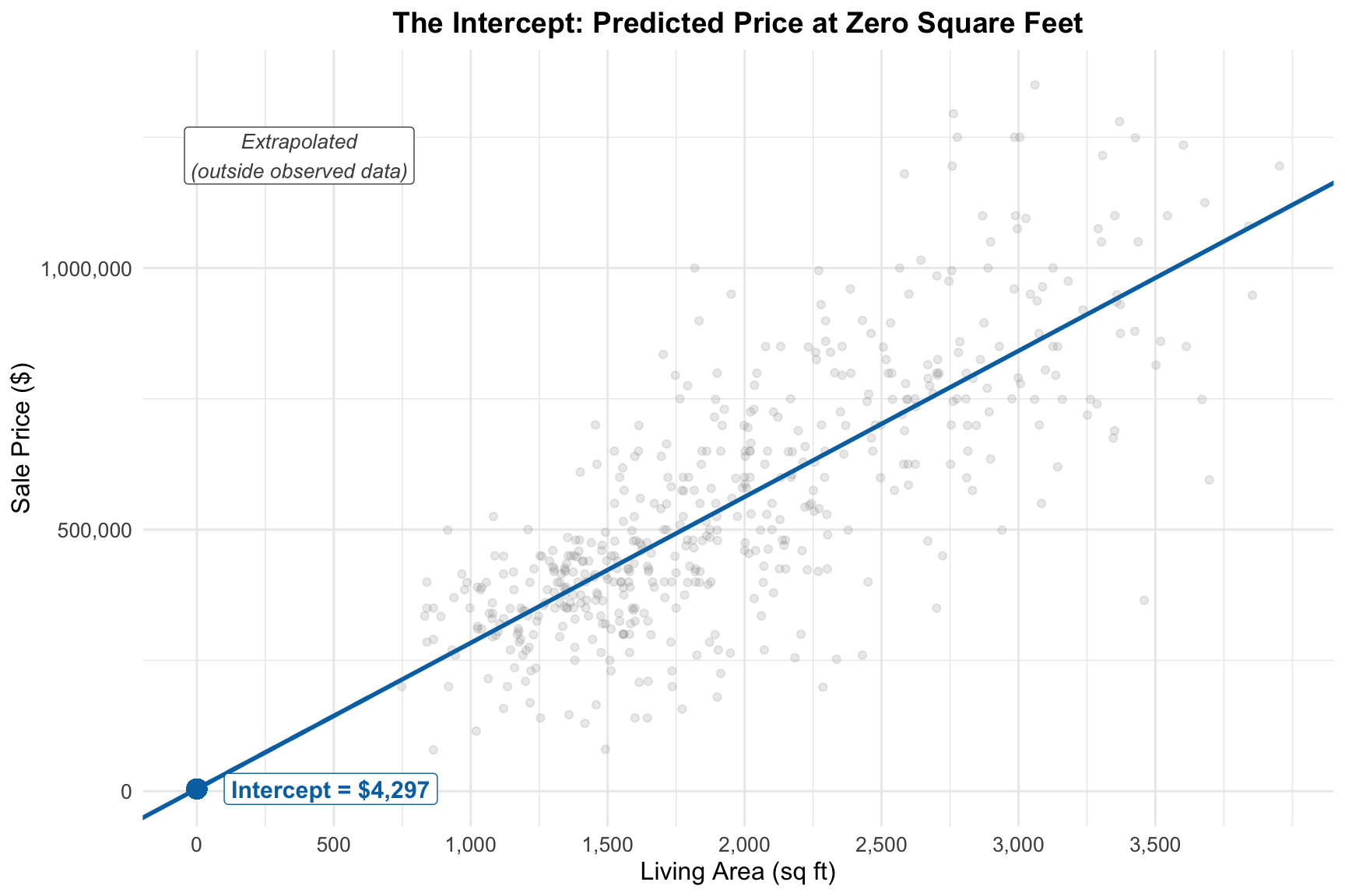
The intercept $\hat\beta_0 = 4,297$ is the predicted price when area equals zero.
In general, the intercept is always our predicted value when $x=0$

Visualizing the intercept

Is the intercept meaningful?

In this example, the intercept has no practical interpretation. We can’t have a house with zero square feet
It’s just an anchor point for the line to put it in the “right” place

When intercepts are meaningful

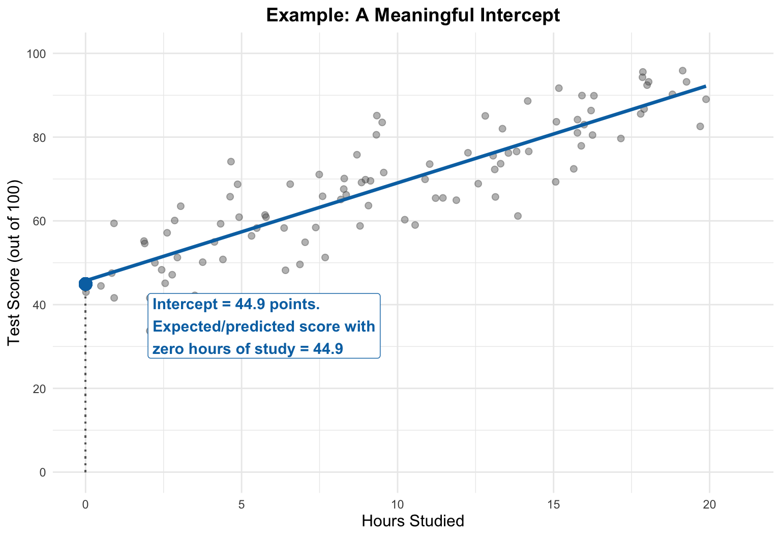
The intercept can be meaningful when zero is a reasonable value for the explanatory variable.
Suppose we were modeling test scores as a function of hours studied…

A meaningful intercept

Uncertainty in coefficients

Like sample means/proportions/differences, our estimates $\hat{\beta}_0$ and $\hat{\beta}_1$ vary from sample to sample
Their standard errors quantify this uncertainty.
The standard error for the slope in this model is $s_{\hat\beta_1} = 10.1$ (from Excel)

Statistical Inference

95% confidence interval for slope:

Same recipe: estimate $\pm$ 2(standard error)
279.4 $\pm$ 2(10.1) = [259.2, 299.6]

This is the set of plausible values.

Hypothesis testing

$\beta_1=0$ is an important possible value for the true parameter: Indicates no linear relationship.
We already saw 0 isn’t a plausible value
Hypothesis test: $H_0: \beta_1 = 0$ vs $H_A: \beta_1 \neq 0$

\[t = \frac{279.14}{10.1} = 27.63\]

p-value < 0.00001
Strong evidence of a linear relationship

Use 2: Prediction

We’ve already seen that once we have a fitted model, we can predict $y$ for new values of $x$:

\[\hat{y}_{\text{new}} = \hat{\beta}_0 + \hat{\beta}_1 x_{\text{new}}\]

For a 2000 sq ft home: \[\hat{y} = 4297 + 279.14 \times 2000 = \$562,576\]

How do we quantify prediction errors?

The residual standard error

The residual standard error $s_e$ = $155,627$ estimates $\sigma$, the standard deviation of prediction errors
Measures the typical size of the residuals.

It tells us how much individual observations deviate from the fitted line (in the same units as $y$).

Prediction Intervals

If our residuals are normally distributed, a 95% prediction interval is \[\widehat{\text{price}} \pm 2s_e = 562,576 \pm 311,255\]

= (251,321, 873,830)

Prediction Intervals

If our residuals are normally distributed, a 95% prediction interval is \[\widehat{\text{price}} \pm 2s_e = 562,576 \pm 311,255\]

= (251,321, 873,830)

Prediction Intervals

Interpretation:

95% of all 2000 sqft houses have sale prices in the range (251,321, 873,830)**
There is a 95% chance (0.95 probability) that a single 2000 sqft house will have a sale price in this range

Application 3: Measuring Relationship Strength

How much does knowing X improve our predictions?

Compare two approaches:

Null model: Predict $\bar{y}$ for everyone
Regression model: Use the fitted line

Null Model vs Regression Model

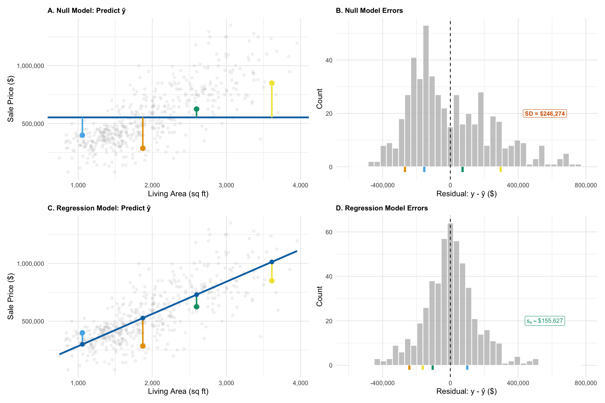
Using area to predict reduces prediction uncertainty (error)

Variance of $y$ = variance of $y-\bar y \approx 246274^2$ ($s^2_y$)
Variance of residuals = variance of $y-\hat y\approx 155,627^2$ ($s^2_e$)
Using $x$ in a linear model produces average squared error that is 40% of the average squared error ignoring $X$ ($\frac{155627^2}{246274^2}\approx 0.4$)
60% of the “unpredictability” in prices goes away when I use area in a linear model

R²: Proportion of Variance Explained

\[R^2 = 1 - \frac{s_e^2}{s_y^2} = 1 - \frac{\text{variance of residuals}}{\text{variance of } y} = 0.6\]

Interpretation: 60% of the variation in house prices is “explained” by the linear relationship with living area.

Range: 0 ≤ R² ≤ 1

R² = 0: X provides no information about Y
R² = 1: Perfect linear fit

Relationship to correlation

For simple linear regression: $R^2 = \text{Cor}(x,y)^2$
- Strength of the linear relationship between $x$ and $y$, irrespective of direction (positive or negative)
For any linear regression: $R^2 = \text{Cor}(\hat y,y)^2$
- Strength of the linear relationship between predicted values $\hat y$ and actual values $y$

High R² doesn’t mean the model is “good”

A high R² doesn’t guarantee:

The relationship is causal
The model is appropriate
Predictions will be accurate
The relationship will continue outside the data

High R² doesn’t mean the model is “good”

Always remember R² is a relative measure:

Our R² is about 0.6, which is pretty high for regression with one variable
But our residual standard error is $155,627$!
Our prediction intervals are probably still too wide for most purposes
Area contains a lot of information about price, but not enough to make this model useful for prediction

Use 4: Adjusted comparisons

Residuals represent deviations from the fitted line—they tell us which observations are above or below what we’d predict based on $x$.
This allows us to make adjusted comparisons: comparing units after accounting for differences in $x$.

Residuals as adjusted comparisons

Residuals = $y_i - \hat{y}_i$ represent how far each observation is from what we’d expect based on the model.

This allows us to identify:

Which houses sold for more/less than predicted
Which observations are unusual
Patterns the model missed

Making adjusted comparisons

Residuals enable “apples-to-apples” comparisons:

Two Austin homes:

House A: 1,703 sq ft, sold for $835,000
House B: 3,670 sq ft, sold for $749,000

Who got the better deal?

Residual Analysis

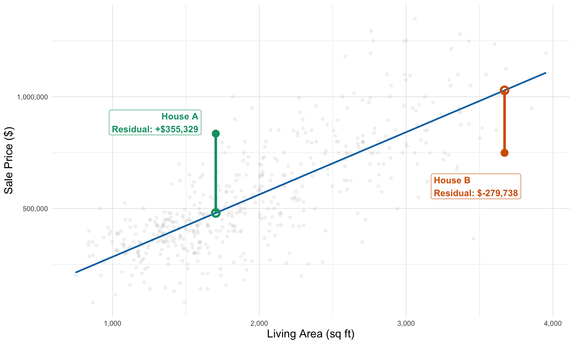
House A: Sold for $355,000 MORE than predicted
House B: Sold for $280,000 LESS than predicted

Residual Analysis

Residuals include:

Unpredictable variation (who is in the market, buyer/seller motivation, condition of neighboring homes)
Predictable variation based on information we have:
- Location
- Age of the home
- Beds, baths, etc
- …

Location

Other notable differences

House A: Downtown proximity, newer construction (2008), spa, garage
House B: Suburban location, older home (1973), no garage

Comparing residuals lets us compare the price of the two houses even though they’re different sizes
To understand which sale was a better value, we’d need a model that accounts for location, amenities, and other factors that “explain” deviation from expected sale price

The Market Model

Example: The market model in finance

The market model relates individual stock returns to market returns:

\[R_{\text{stock}} = \alpha + \beta \times R_{\text{market}} + \epsilon\]

This is just linear regression applied to financial returns. Let’s see how to interpret $\alpha$ and $\beta$

Market model notation

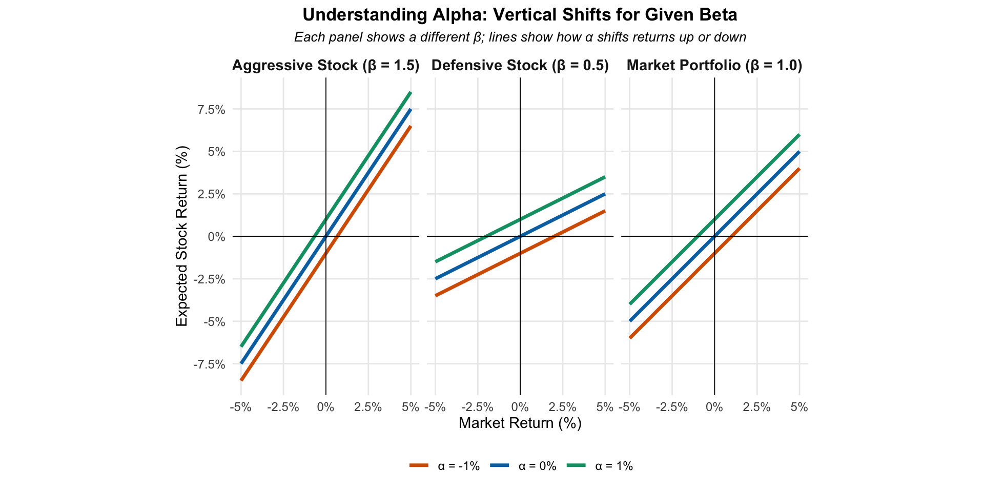
$\beta$ (slope): beta or market sensitivity—how much the stock moves with the market (on average)
- Aka: Sysetmic/market risk
$\alpha$ (intercept): alpha or excess return — average excess (market) risk-adjusted return
- Comparing stocks with the same $\beta$, higher $\alpha$ means better returns on average
Residuals: company-specific returns not explained by market movements

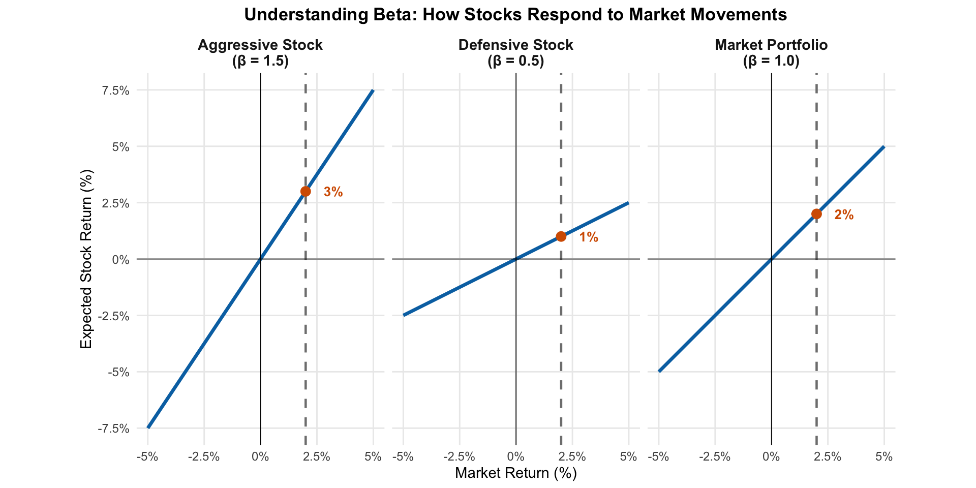
What beta means

$\beta < 1$: Stock is less volatile than the market (defensive)
$\beta = 1$: Stock moves in line with the market
$\beta > 1$: Stock is more volatile than the market (aggressive/cyclical)

What alpha means

$\alpha$ is the expected return when the market is flat (x=0 means a 0% SP500 return)
Usually close to zero for accessible investments
$\alpha$ is the (expected) excess risk-adjusted return
- Comparing two investments with the same $\beta$, the one with higher $\alpha$ has higher expected returns under all market conditions

What alpha means

Apple vs S&P 500

Interpreting beta

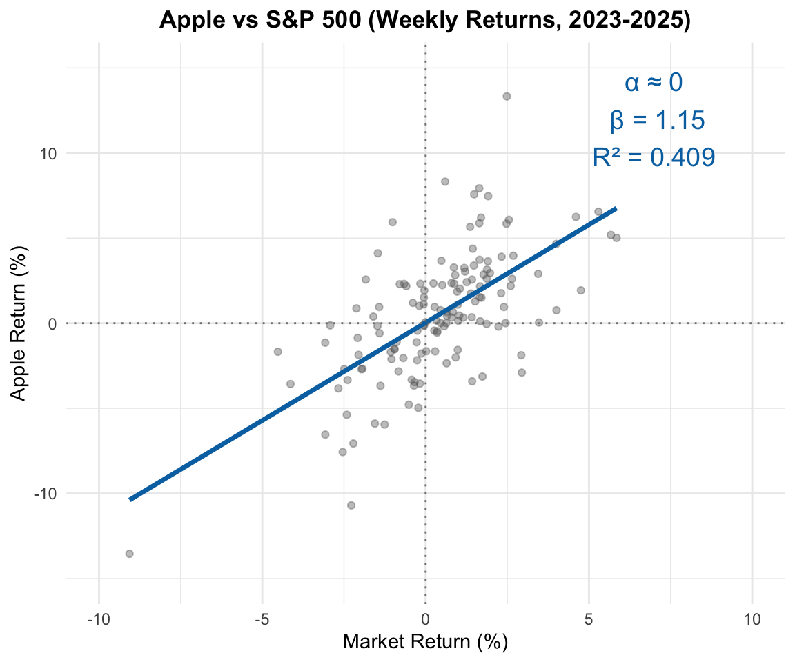
Apple’s $\beta$ = 1.15 means:

When the market goes up by 1%, we expect Apple to go up by about 1.15% on average.
Since $\alpha\approx 0$, across all days when the market is up 1% on average the Apple return is about 1.15%

Beta measures market sensitivity or systematic risk.

Different betas

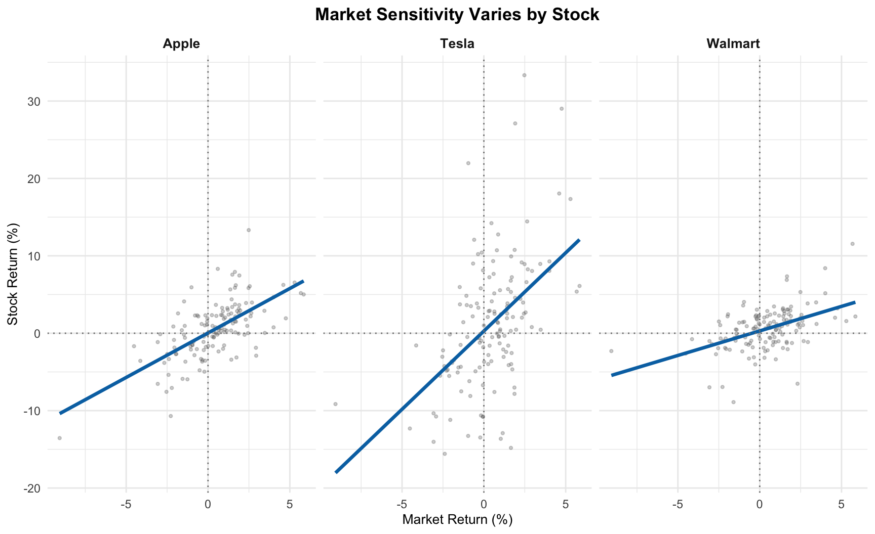
Different stocks have different market sensitivities:

Apple: $\beta$ = 1.15
Tesla: $\beta$ = 2.02
Walmart: $\beta$ = 0.63

Comparing betas

Accounting for uncertainty: Tesla

From a fitted market model for Tesla:

Parameter	Estimate	Std Error
$\alpha$ (intercept)	0.284%	0.626%
$\beta$ (slope)	2.022	0.3

These are estimates of the true parameters; we need to account for uncertainty.

Confidence intervals for Tesla

95% confidence intervals (estimate $\pm$ 2 standard errors):

Alpha (excess return):

0.284 $\pm$ 2 × 0.626 = [-0.969%, 1.537%]

Beta (market sensitivity):

2.022 $\pm$ 2 × 0.3 = [1.422, 2.621]

Testing alpha = 0

Null hypothesis: $H_0: \alpha = 0$ (no excess risk-adjusted returns)

Test statistic: \[t = \frac{\hat{\alpha} - 0}{s_{\hat{\alpha}}} = \frac{0.284}{0.626} = 0.453\]

p-value: 0.6504

Testing beta = 1

Null hypothesis: $H_0: \beta = 1$ (market-equivalent systematic risk)

Test statistic: \[t = \frac{\hat{\beta} - 1}{s_{\hat{\beta}}} = \frac{2.022 - 1}{0.3} = 3.409\]

p-value: 0.0009

Interpreting the beta test

With p = 0.0009, we reject the null hypothesis at the 5% level.
Coupled with the 95% CI that only includes positive values, we can conclude with confidence that TSLA stock has $\beta>1$

Slope vs correlation/R²

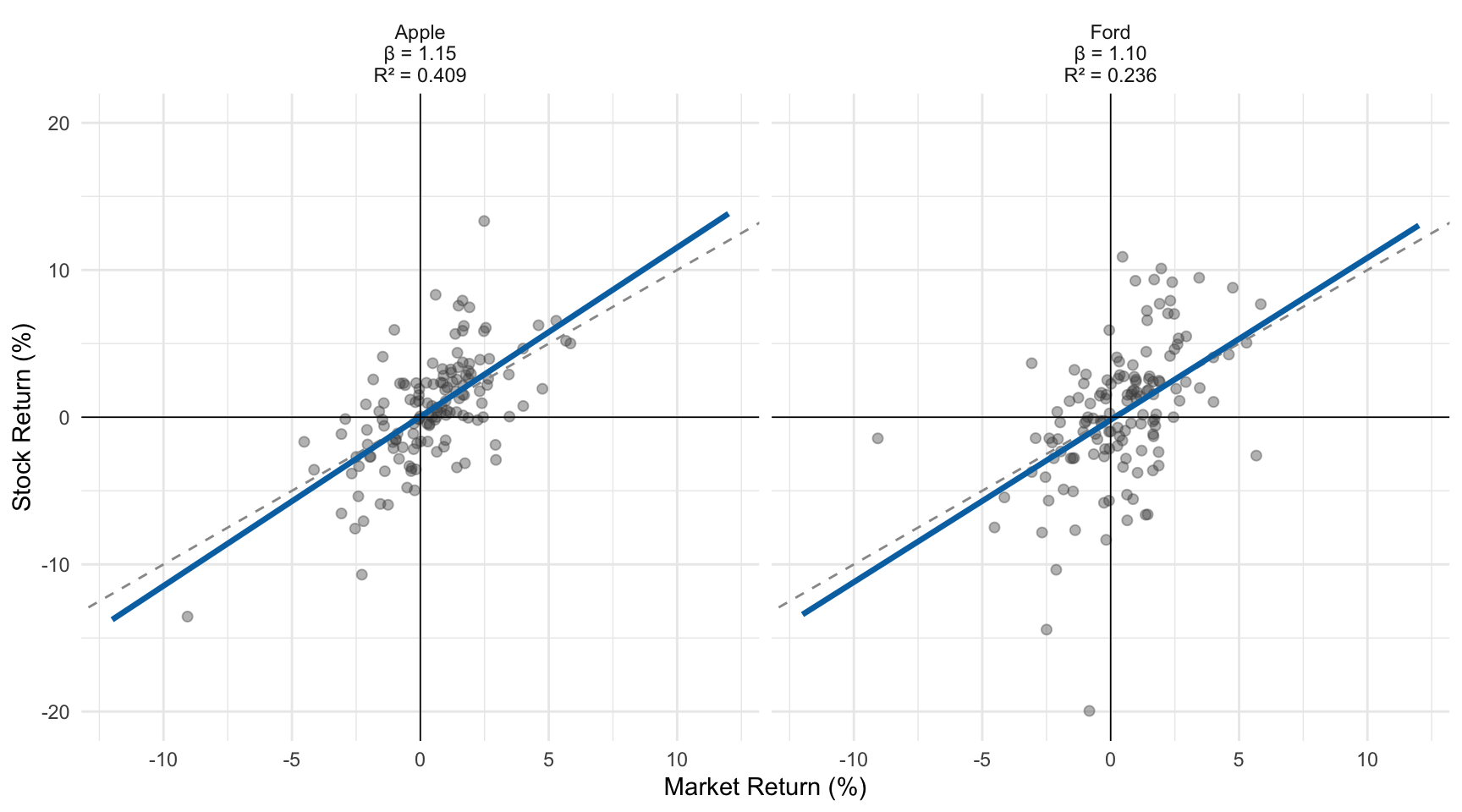
Two stocks can have the same slope ($\beta$) but very different R² values, or the same R² but different slopes
High $\beta$ does NOT mean high correlation between stock and market returns, and low R² does NOT mean low market risk

Similar Slopes (Betas), Different R²

These stocks have similar market sensitivity (betas), but very different R²— Ford has more company-specific volatility that isn’t predicted by market movements.
We see this as increased spread around the fitted line, since the standard deviation of AAPL and Ford returns are similar (3.6% and 4.6%)

Tesla vs Ford Market Models

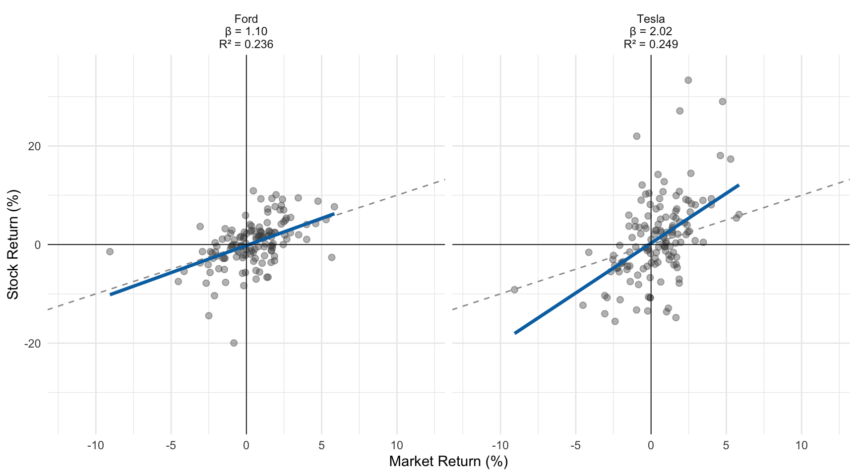
Similar Slopes (Betas), Different R²

These stocks have similar $R^2$ but very different market sensitivity (betas)
But remember, $R^$ is relative
- TSLA’s residual standard error (7.2%) is much higher than Ford’s (4.1%)
- We get similar $R^2$ because TSLA has more overall volatility (higher SD/variance of returns – more spread along y-axis)

Residuals as market-adjusted returns

The residuals from the market model represent returns that cannot be explained by overall market movements—these are company-specific or industry-specific shocks.

Tesla residuals over time

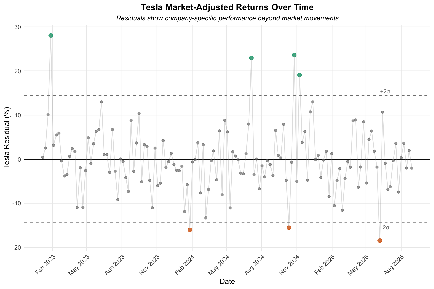
Tesla’s Extreme Events

Large Negative Residual (June 2025):

Public feud between Musk and President Trump
Company-specific risk unrelated to market performance

Large Positive Residual (July 2024):

Stronger than expected car deliveries
Approval of CEO compensation package
Positive news = better than expected returns