Call:
lm(formula = diagmath_spring_s ~ treatment + block, data = tutoring)
Residuals:
Min 1Q Median 3Q Max
-4.297 -0.737 0.095 0.683 2.905
Coefficients:
Estimate Std. Error t value Pr(>|t|)
(Intercept) 0.02638 0.12007 0.22 0.8262
treatment 0.07223 0.09174 0.79 0.4315
blockgrade6.wave2 -0.09601 0.16636 -0.58 0.5641
blockgrade6.wave3 -0.00421 0.22160 -0.02 0.9848
blockgrade7.wave1 -0.03603 0.16285 -0.22 0.8250
blockgrade7.wave2 -0.13626 0.18135 -0.75 0.4528
blockgrade7.wave3 -0.19781 0.26389 -0.75 0.4539
blockgrade8.wave1 0.12562 0.15642 0.80 0.4223
blockgrade8.wave2 0.14897 0.16570 0.90 0.3691
blockgrade8.wave3 -0.63119 0.23136 -2.73 0.0066 **
---
Signif. codes: 0 '***' 0.001 '**' 0.01 '*' 0.05 '.' 0.1 ' ' 1
Residual standard error: 1.02 on 487 degrees of freedom
(63 observations deleted due to missingness)
Multiple R-squared: 0.0294, Adjusted R-squared: 0.0114
F-statistic: 1.64 on 9 and 487 DF, p-value: 0.102Basic causal inference and randomized controlled trials
First strategy for inferring causation: controlling for confounders
Chance, confounders, and colliders
If we run a regression predicting Y from X and find that X is a significant predictor of Y, we might like to conclude that X causes Y. But it might be the case that:
- Y actually causes X.
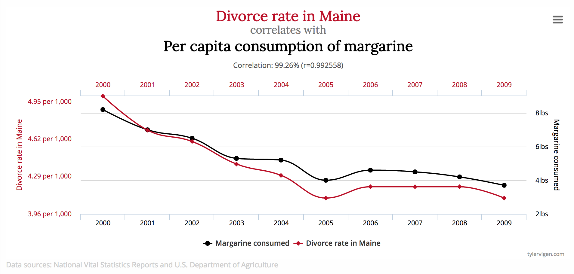
- X and Y are not actually related in the population; they happen to be correlated in the sample just by chance.
- A common variable Z (a confounder) causes both X and Y.
- A common variable W (a collider) is caused by both X and Y.
Spurious (chance) correlations
Confounders (lurking variables)
A confounder is a third variable that causes both X and Y and explains the observed correlation between X and Y:
- Days on which more ice cream is consumed tend to also have higher crime.
- People who are vaccinated against COVID-19 are 34% less likely to die from non-COVID causes, compared to unvaccinated people.
Colliders
A collider is a third variable that is caused by both X and Y.
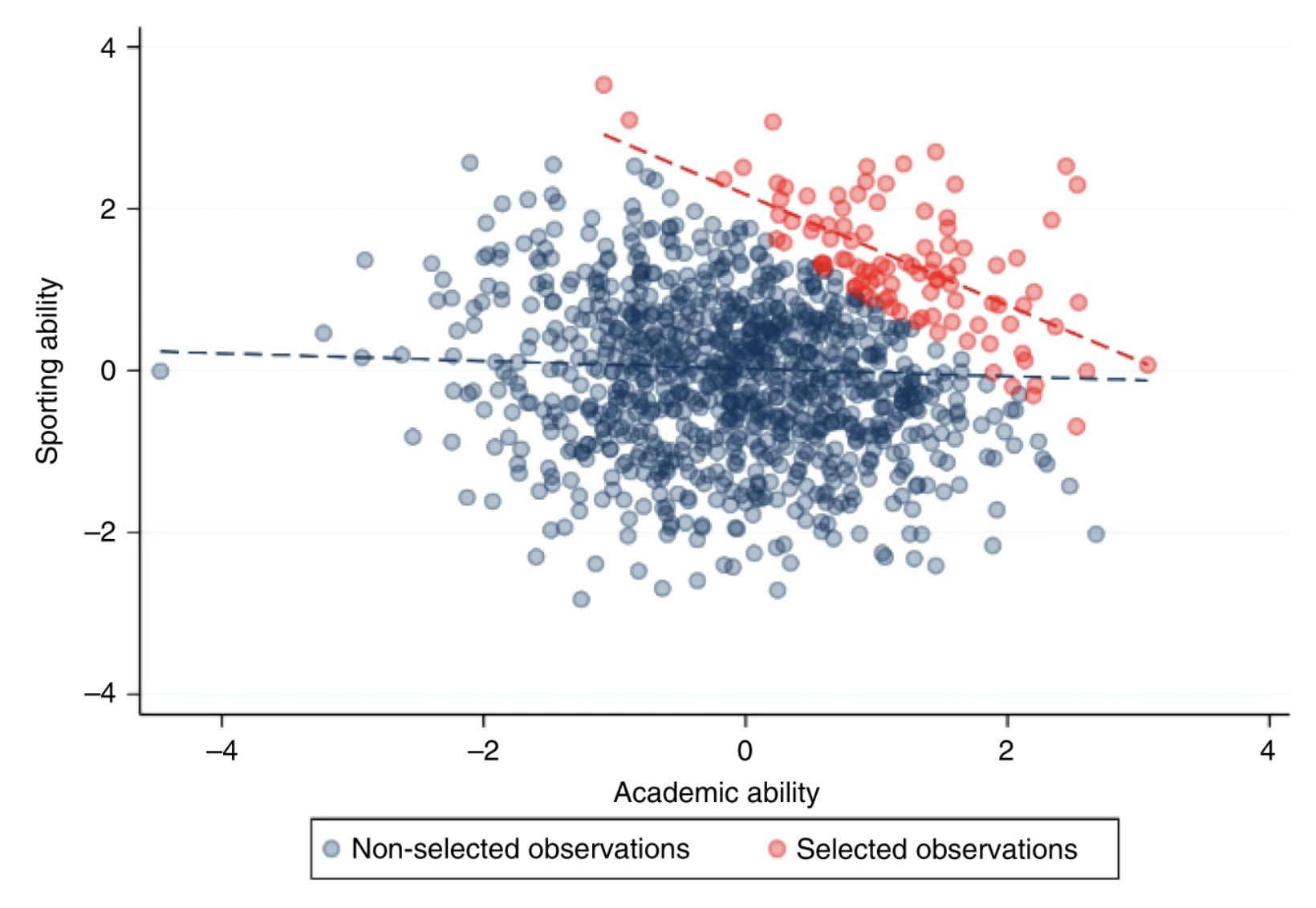
- Talent and attractiveness is negatively correlated among celebrities even if uncorrelated in general
- You become a celebrity if you are really good at something or really good-looking (maybe, but not usually, both), so most celebrities have one but not the other
Colliders
A collider is a third variable that is caused by both X and Y.
Among hospitalized patients, smokers are less likely to have COVID than non-smokers
- Both COVID and smoking make you more likely to land in the hospital, so if you are a smoker you probably got there because of smoking, not COVID
Selecting the sample using a collider can change the correlation!
Colliders
Using regression to try to infer causation (last week)
- Control for potential confounders so the slope of X expresses the “partial” relationship between X and Y without the effect of the confounder mixed in.
- Example: Predict crime rate from ice cream consumption, but control for temperature.
- Do not control for colliders because doing so might mislead us about the nature of the relationship between X and Y.
- But this strategy is not perfect: we cannot be sure that we have controlled for all possible confounders!
Randomized Controlled Trials
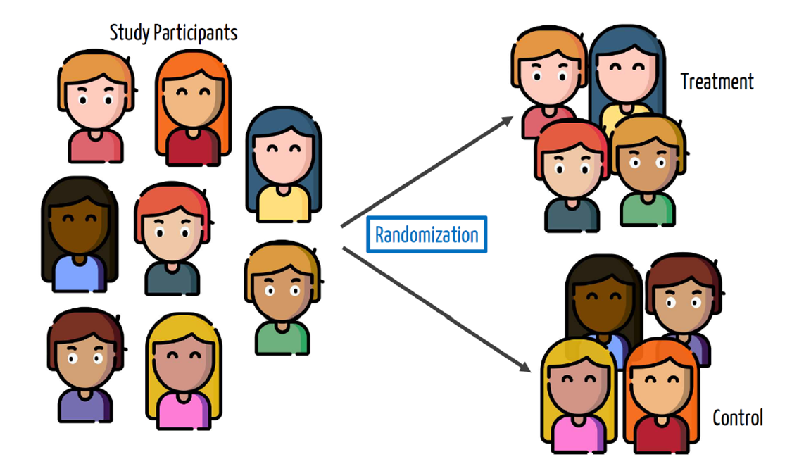
Randomized controlled trials (RCTs)
- Often called the “gold standard” for establishing causality
- Randomly assign the value of X to participants
- Now, any observed relationship between X and Y must be due to X, since the only reason an individual had a particular value of X was the random assignment
Why does randomization work?
- Randomization ensures that the treatment and control groups are, on average, identical in all respects except for the treatment itself.
- Put another way: if Z is a binary treatment dummy, then it’s (approximately) uncorrelated with any other variable in or out of the dataset
- The regression coefficient on Z – difference in averages between treatment and control groups – is about the same whether or not we include additional variables!
Common business applications of RCTs
- Marketing: A/B testing to see which version of an mail marketing campaign performs better
- Management: Testing out a sales bonus structure by randomly assigning stores to bonus plans
- MIS: Randomly segmenting a small % web traffic to a new server that is being tested
The fundamental problem of causal inference
Suppose you have a headache, and you take an asprin. Then you don’t have a headache. Did the asprin work?
The fundamental problem of causal inference
For any given person, we can only observe one outcome or the other, depending on whether the person took an asprin or not:
| Person | Took asprin | Didn’t take asprin |
|---|---|---|
| 1 | no headache | ? |
| 2 | no headache | ? |
| 3 | no headache | ? |
| 4 | no headache | ? |
| 5 | ? | no headache |
| 6 | ? | headache |
| 7 | ? | headache |
| 8 | ? | headache |
Solving the fundamental problem of causal inference
The best we can do is compute an average treatment effect: the difference in the statistic of interest between the treatment vs control group:
\begin{align*} \text{Average treatment effect} &= (\% \text{ headache among asprin-takers}) - {} \\ &\qquad (\% \text{ headache among non-asprin-takers}) \\ &= 0/4 - 3/4 \\ &= -0.75 \end{align*}
Example 1: Phase 3 Clinical Trial for the Moderna COVID-19 vaccine
- X = got the vaccine, Y = got COVID-19
- Randomly assign study participants to get either the vaccine (a treatment group of 14,134 people) or a placebo (a control group of 14,073 people)
- 11 vaccine recipients got COVID; 185 of placebo recipients got COVID
Threats to validity
Two types of validity
- Internal validity is the ability of an experiment to establish cause-and-effect of the treatment within the sample studied.
- External validity is the ability of an experimental result to generalize to a larger context or population.
Two types of validity
Example: Randomly assign salespeople to one of two different compensation plans, and measure their sales performance over the next year.
- Internal validity: We can conclude that the choice of compensation plan caused the difference in sales performance.
- External validity: We can conclude that the same choice of compensation plan would have a similar impact in other salespeople outside of our sample.
What is a threat to validity?
A threat to validity is something that, if true, would cause us to doubt the conclusion that a particular study comes to.
Internal validity
Internal validity is the ability of an experiment to establish cause-and-effect of the treatment within the sample studied.
Examples of threats to internal validity:
- Failure to randomize
- Failure to follow the treatment protocol / attrition
- Small sample sizes
External validity
External validity is the ability of an experimental result to generalize to a larger context or population.
Examples of threats to external validity:
- Nonrepresentative samples
- Nonrepresentative protocol/policy
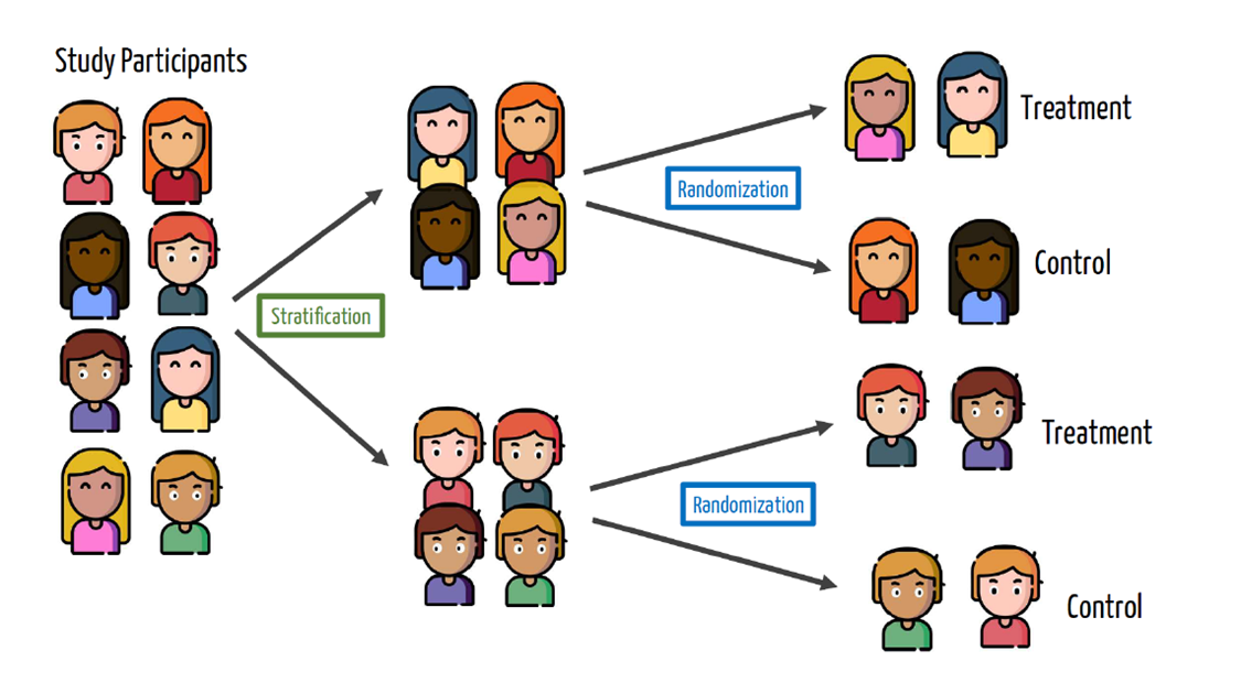
Using blocking to improve validity
Using blocking to improve validity
- Randomization works “on average” (i.e., if we were able to run the experiment many times) but we only get one shot at creating treatment and control groups, and there might be imbalances in “nuisance” variables that could affect the outcome.
- For example, what will happen if the treatment group for the Moderna trial happens to get younger people in it than the control group?
- We can solve this by blocking: randomly assigning to treatment/control within groups
Without blocking: gender imbalance, due to random chance
With blocking: perfect gender balance, by design
Blocking in the Moderna vaccine trial
In the Moderna vaccine trial, they identified two possible variables that could impact COVID outcomes:
- Age (65+ vs under 65)
- Underlying health condition
Blocking design for Moderna trial
Everyone
├── Age 65+
│   ├── Healthy
│   │   ├── Treatment (Randomize)
│   │   └── Control (Randomize)
│   └── Underlying condition
│       ├── Treatment (Randomize)
│       └── Control (Randomize)
└── Age <65
    ├── Healthy
    │   ├── Treatment (Randomize)
    │   └── Control (Randomize)
    └── Underlying condition
        ├── Treatment (Randomize)
        └── Control (Randomize)
Analyzing experiments using regression
- For non-blocked design, use a simple regression (T = dummy variable that is 1 for treatment group and 0 for control group): \hat Y = \hat\beta_0 + \hat\beta_1 T
- For a blocked design, use a regression that controls for the blocking variable B: \hat Y = \hat\beta_0 + \hat\beta_1 T + \hat\beta_2 B
In both cases, the coefficient of T (\hat\beta_1) represents the estimated average treatment effect. The regression needs to be logistic if Y is categorical!
Example 2: Does online tutoring improve student achievement?
- Kraft, List, Livingston, and Sadoff (2022) study a pilot program in which volunteer college tutors met 1-on-1 online with middle-school students during the school day.
- Students from Chicago Heights Middle School in spring 2021, during the transition from fully remote instruction to hybrid learning.
- Eligible students were those who chose hybrid learning; a total of 560 students were randomized.
- The treatment was online tutoring two days per week for 30 minutes during advisory period.
- The main outcomes Y are standardized math and reading test scores
Example 2: Online tutoring by college volunteers
The study used blocking because treatment was rolled out across three waves, and randomization was done by grade level (to ensure proportional allocation).
- Wave 1: March 8 (n=268)
- Wave 2: March 22 (n=209)
- Wave 3: April 5 (n=83)
- Within each wave, students were randomized separately by grade level
So the analysis controls for wave-by-grade randomization blocks.
Blocking design for tutoring experiment
Hybrid-learning students eligible for study
├── Wave 1 entrants
│   ├── Grade 6: Treatment vs Control (Randomize)
│   ├── Grade 7: Treatment vs Control (Randomize)
│   └── Grade 8: Treatment vs Control (Randomize)
├── Wave 2 entrants
│   ├── Grade 6: Treatment vs Control (Randomize)
│   ├── Grade 7: Treatment vs Control (Randomize)
│   └── Grade 8: Treatment vs Control (Randomize)
└── Wave 3 entrants
    ├── Grade 6: Treatment vs Control (Randomize)
    ├── Grade 7: Treatment vs Control (Randomize)
    └── Grade 8: Treatment vs Control (Randomize)
Analyzing the tutoring experiment
Analyzing the tutoring experiment
                   2.5 % 97.5 %
(Intercept)       -0.210  0.262
treatment         -0.108  0.252
blockgrade6.wave2 -0.423  0.231
blockgrade6.wave3 -0.440  0.431
blockgrade7.wave1 -0.356  0.284
blockgrade7.wave2 -0.493  0.220
blockgrade7.wave3 -0.716  0.321
blockgrade8.wave1 -0.182  0.433
blockgrade8.wave2 -0.177  0.475
blockgrade8.wave3 -1.086 -0.177
Analyzing the tutoring experiment
- The estimated effect of offering tutoring is about 0.072$ standard deviations on the math test.
- The 95% confidence interval for the effect ranges from about -0.108$ to 0.252$ standard deviations.
- Adjusting for other controls (e.g., pre-treatment test scores) does not change the estimated effect much, but it does reduce the standard error and make the confidence interval narrower.
Analyzing the tutoring experiment
Call:
lm(formula = diagmath_spring_s ~ treatment + math_s + reading_s +
    block, data = tutoring)

Residuals:
    Min      1Q  Median      3Q     Max
-1.8353 -0.4003  0.0164  0.3713  2.2897

Coefficients:
                  Estimate Std. Error t value             Pr(>|t|)
(Intercept)         0.0761     0.0750    1.01                0.311
treatment           0.0653     0.0573    1.14                0.255
math_s              0.6325     0.0420   15.07 < 0.0000000000000002 ***
reading_s           0.2341     0.0427    5.48          0.000000068 ***
blockgrade6.wave2  -0.0951     0.1042   -0.91                0.362
blockgrade6.wave3  -0.0169     0.1383   -0.12                0.903
blockgrade7.wave1  -0.0888     0.1017   -0.87                0.383
blockgrade7.wave2  -0.1945     0.1132   -1.72                0.086 .
blockgrade7.wave3  -0.2592     0.1648   -1.57                0.116
blockgrade8.wave1  -0.0147     0.0981   -0.15                0.881
blockgrade8.wave2   0.0902     0.1034    0.87                0.384
blockgrade8.wave3  -0.2757     0.1450   -1.90                0.058 .
---
Signif. codes:  0 '***' 0.001 '**' 0.01 '*' 0.05 '.' 0.1 ' ' 1

Residual standard error: 0.635 on 485 degrees of freedom
  (63 observations deleted due to missingness)
Multiple R-squared:  0.624, Adjusted R-squared:  0.615
F-statistic:   73 on 11 and 485 DF,  p-value: <0.0000000000000002
Analyzing the tutoring experiment
                    2.5 %  97.5 %
(Intercept)       -0.0713 0.22346
treatment         -0.0473 0.17801
math_s             0.5501 0.71504
reading_s          0.1502 0.31804
blockgrade6.wave2 -0.2999 0.10975
blockgrade6.wave3 -0.2887 0.25484
blockgrade7.wave1 -0.2887 0.11111
blockgrade7.wave2 -0.4169 0.02797
blockgrade7.wave3 -0.5830 0.06461
blockgrade8.wave1 -0.2075 0.17804
blockgrade8.wave2 -0.1131 0.29343
blockgrade8.wave3 -0.5607 0.00927
Results from the tutoring experiment
- Intent-to-treat (pooled across tests): about 0.07 SDs for math
- Effects are positive but statistically insignificant in this pilot study
- Estimates are larger in Wave 1 than in Waves 2 and 3, consistent with a possible dosage effect
- Students attended about 3.1 hours of tutoring on average; later waves had fewer chances to attend
Wave 1 results
Call:
lm(formula = diagmath_spring_s ~ treatment + factor(grade), data = tutoring %>%
    filter(wave == 1))

Residuals:
    Min      1Q  Median      3Q     Max
-2.4194 -0.6673  0.0958  0.6689  2.2251

Coefficients:
               Estimate Std. Error t value Pr(>|t|)
(Intercept)     -0.0199     0.1227   -0.16     0.87
treatment        0.1616     0.1243    1.30     0.19
factor(grade)7  -0.0345     0.1544   -0.22     0.82
factor(grade)8   0.1251     0.1483    0.84     0.40

Residual standard error: 0.964 on 237 degrees of freedom
  (27 observations deleted due to missingness)
Multiple R-squared:  0.0123,    Adjusted R-squared:  -0.000174
F-statistic: 0.986 on 3 and 237 DF,  p-value: 0.4
Wave 1 results
Call:
lm(formula = diagmath_spring_s ~ treatment + math_s + factor(grade),
    data = tutoring %>% filter(wave == 1))

Residuals:
    Min      1Q  Median      3Q     Max
-1.7841 -0.3600  0.0079  0.3581  1.6179

Coefficients:
               Estimate Std. Error t value            Pr(>|t|)
(Intercept)      0.0331     0.0775    0.43                0.67
treatment        0.0984     0.0784    1.25                0.21
math_s           0.7952     0.0419   18.97 <0.0000000000000002 ***
factor(grade)7  -0.0643     0.0974   -0.66                0.51
factor(grade)8   0.0361     0.0936    0.39                0.70
---
Signif. codes:  0 '***' 0.001 '**' 0.01 '*' 0.05 '.' 0.1 ' ' 1

Residual standard error: 0.608 on 236 degrees of freedom
  (27 observations deleted due to missingness)
Multiple R-squared:  0.609, Adjusted R-squared:  0.602
F-statistic: 91.8 on 4 and 236 DF,  p-value: <0.0000000000000002
Threats to validity of the tutoring experiment?
- What are some possible threats to validity here?
Imperfect uptake
- About 18% of treated students attended no tutoring at all
- Very common!
- Is this a threat to internal or external validity?
Imperfect uptake
- It is a threat to internal validity if we want the effect of tutoring itself
- But we can still get an internally valid estimate of the effect of being offered tutoring (the intent-to-treat effect)
- This often answers a more policy-relevant question anyway
The tutor pool
- Tutors were unpaid volunteers, many from highly selective colleges (including UT!)
- To scale up, the program would need many more tutors – might need to offer pay, or be less selective
- Is this a threat to internal or external validity?
The tutor pool
- It is a threat to external validity – how would the treatment work in a broader population?
- Not a threat to internal validity – the estimated effect of offering tutoring is still valid for the sample studied, even if the tutors were unusually good
The student pool
- This was a single pilot program in one Chicago middle school during the COVID-19 pandemic
- Would we see the same effect in rural schools in 2026?
The student pool
- This is a threat to external validity – the results may not generalize to other settings, grades, districts, or non-pandemic environments
- Not a threat to internal validity
- It is common for pilot studies to have limited external validity before conducting larger-scale trials with more representative samples
The limitations of RCTs
Although they are powerful for inferring causation, RCTs are hard to pull off:
- They can be incredibly expensive (e.g., Phase 3 clinical trial)
- Compliance with the treatment protocol isn’t perfect
- It can be hard to generalize beyond the participants involved in the study, if they aren’t representative (e.g., psychology experiments conducted on college students)
- They can be impractical (e.g., effect of education on performance) or unethical to conduct (e.g., seatbelts, parachutes, even some medical trials)